
Your model is only as accurate as its weakest assumption. Train a single model too closely, and it memorizes noise. Keep it too simple, and it misses real patterns. No single model escapes this tension, and a more complex architecture will not necessarily fix it. Ensemble learning methods are the practical answer: combine multiple models strategically, and their individual errors cancel out, leaving predictions that are more reliable than any single contributor can produce. This guide covers the three core ensemble learning methods: bagging, boosting, and stacking, when to use each, how to implement them, and where they deliver the most value in practice.
Key Takeaways
- Single models fail because of the bias-variance tradeoff; ensemble learning methods can address both failure modes in many cases.
- Bagging (e.g., Random Forest) reduces variance through parallel, independent training on bootstrap samples.
- Boosting (e.g., XGBoost, LightGBM) reduces bias through sequential, error-correcting training.
- Stacking trains a meta-learner on base model outputs for the highest possible predictive ceiling.
- Simple voting or averaging can sometimes match stacking at a lower engineering cost.
- Interpretability requirements, latency constraints, and data size all affect which method to pick.
What Are Ensemble Learning Methods?
Ensemble learning methods work by combining the outputs of multiple base models into a single prediction that no individual model could produce alone. Understanding why this works and where it stops working is what separates thoughtful application from mechanical pattern-matching.
Why Combining Models Works
Here is the concrete version of why combining models helps. Suppose you ask five analysts to predict customer churn. Each uses slightly different data and a different approach. Some will be wrong, but they will not all be wrong in the same direction. Average their predictions, and you get something closer to the truth than any single analyst produces. That is ensemble learning.
The mathematics supports this intuition. When models make independent prediction errors with similar variance, averaging reduces variance approximately in proportion to $$1 /N$$. In practice, the gain is smaller when model errors are correlated. In practice, the benefit is limited by the correlation between model errors. Base learners can be anything — decision trees, neural networks, support vector machines, or linear models. What matters is that they differ enough to disagree on at least some examples. That disagreement is what ensemble methods refine into better predictions. [1]
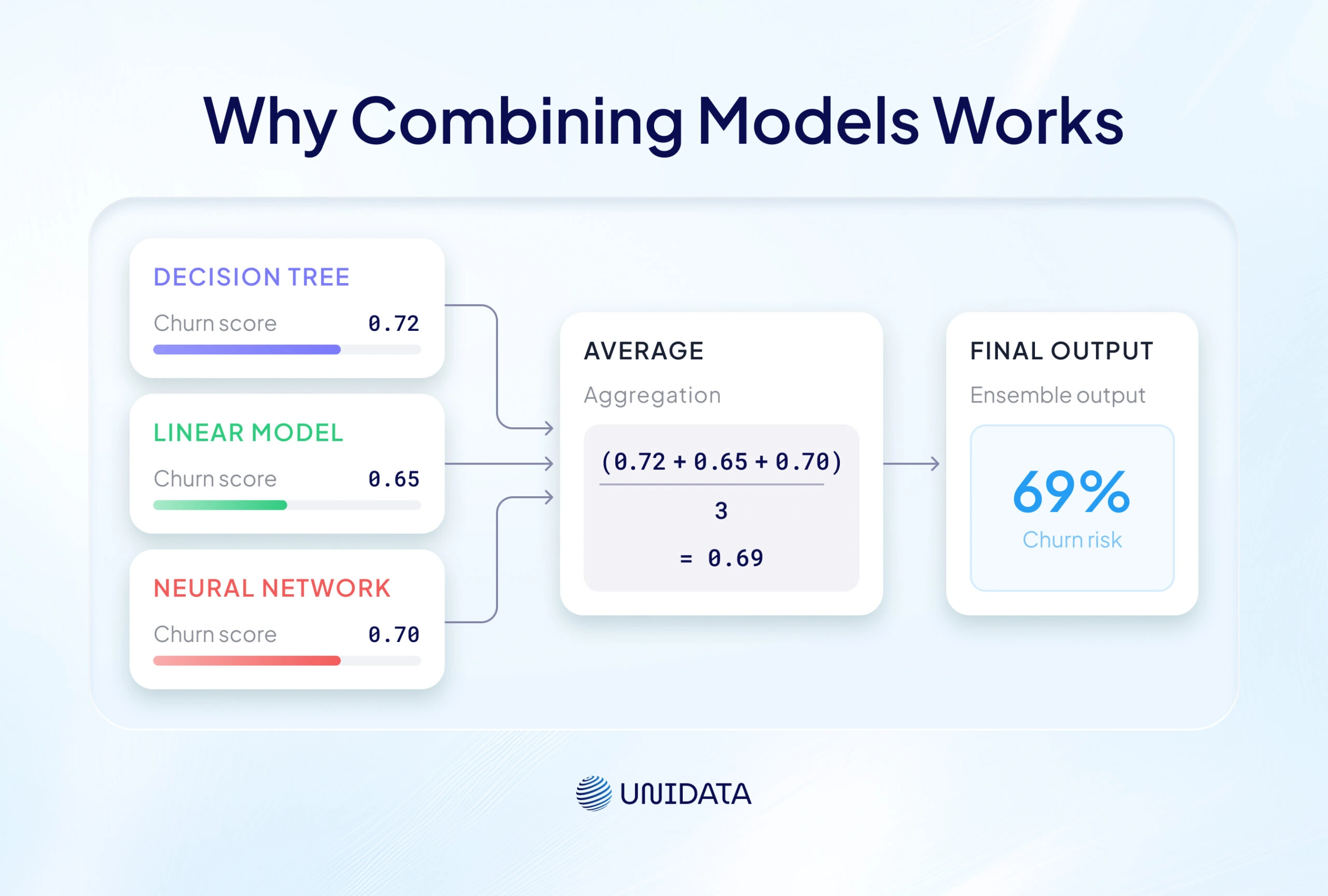
Figure 1: Multiple base model predictions feed into an aggregation layer to produce the ensemble's final output.
How Ensemble Learning Methods Reduce Error. The Bias-Variance Tradeoff
Any model's prediction error breaks into three parts:
$$$\text{Bias}^{2} + \text{Variance} + \text{Irreducible Error}$$$
- Bias is systematic error, meaning that the model consistently misses in the same direction.
- Variance is sensitivity to the training set, meaning that the model changes dramatically when data shifts slightly.
- Irreducible error is noise no model can remove.
The dartboard analogy makes this concrete. High bias means all your darts cluster away from the bullseye. High variance means they scatter randomly. You want tight grouping on the target — low bias and low variance at once.
The two main ensemble learning methods address each error type directly. Bagging primarily reduces variance by training parallel models on different data samples and aggregating their predictions. Boosting reduces bias by training sequential models that each correct the previous one's errors. Identifying which error type dominates your problem is the first design decision. [1]
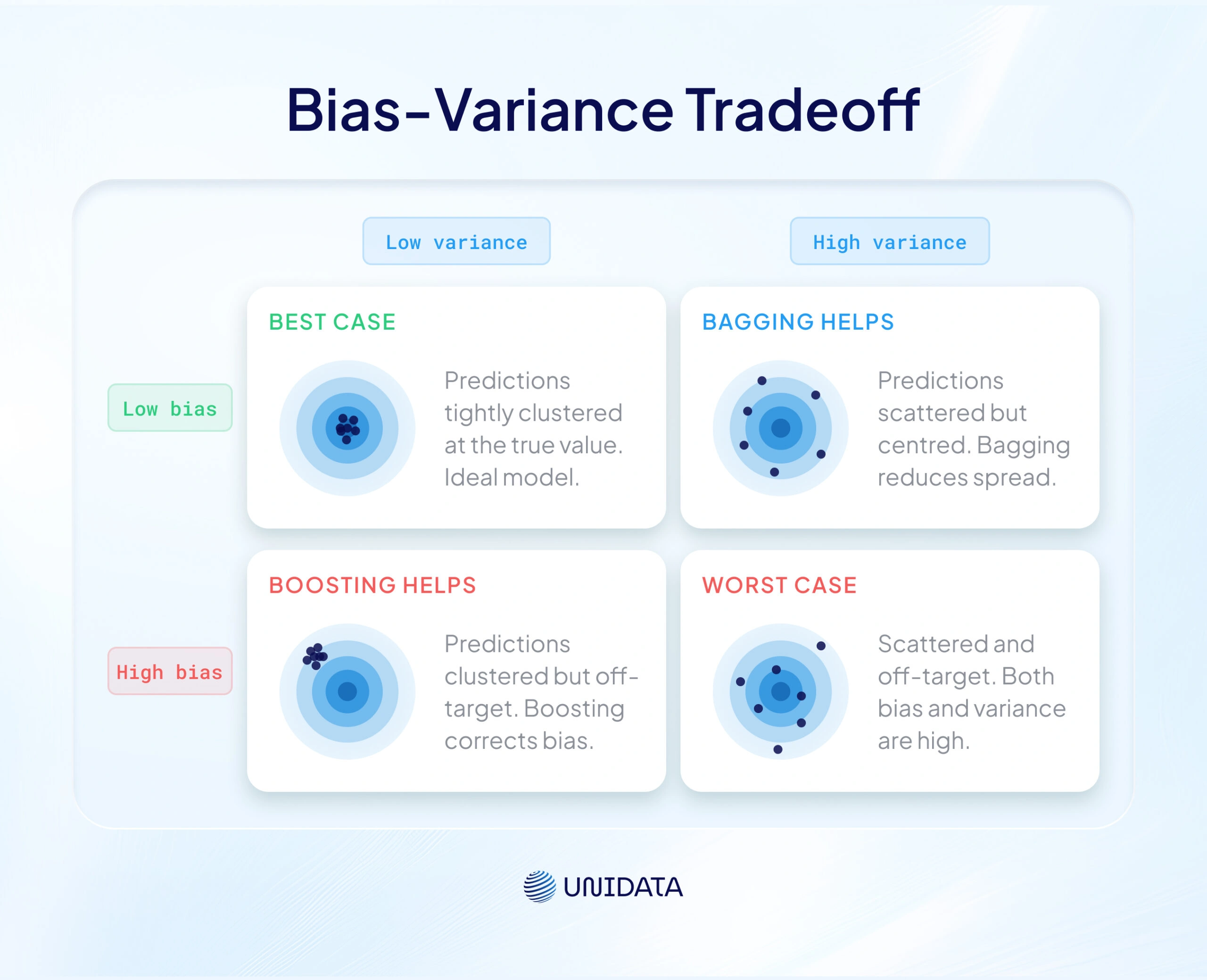
Figure 2: Each dartboard shows a different error profile. Think of the bullseye as the correct answer. Top-left (low bias, low variance) is the goal. Top-right (low bias, high variance) is what you get with an unstable model — bagging fixes this. Bottom-left (high bias, low variance) is a model that consistently guesses wrong — boosting fixes this. Bottom-right is the worst case.
A Brief History: From Bagging to XGBoost
One of the key problems that accelerated interest in modern ensembles was decision tree instability. Small changes in training data produce dramatically different trees. Breiman's 1996 bagging paper offered the first systematic solution, followed by his 2001 Random Forest, which added feature randomness at each split. [1]
On the boosting side, Freund and Schapire's AdaBoost (1997) showed that combining many weak learners could produce a strong predictor. [2] Chen and Guestrin’s XGBoost (2016) scaled and optimized the gradient boosting framework for large-scale production workloads through regularization, efficient tree construction, and distributed training support. [3] LightGBM was released in 2017 with histogram-based approximations that often reduced training time substantially on large datasets.
Key Milestones in Ensemble Learning
Year
1996
1997
2001
2002
2016
2017
Milestone
Breiman publishes Bagging (Bootstrap Aggregating)
Freund & Schapire publish AdaBoost
Breiman introduces Random Forest
Friedman publishes Stochastic Gradient Boosting
Chen & Guestrin release XGBoost (KDD 2016)
Microsoft releases LightGBM
When to Use an Ensemble and When Not To
No single pattern fits every problem. The right choice depends on your error type, your data size, and how much complexity you can afford to maintain.
| Use an Ensemble When… | A Single Model May Be Enough When… |
|---|---|
| The single model has a measurably high variance or bias | Training data is very small, e.g., under 1,000 rows |
| You have sufficient training data (generally > 5,000 rows) | Inference latency is a hard constraint |
| Compute and maintenance costs are acceptable | Regulatory or legal interpretability is required |
| Structured / tabular data with mixed feature types | Feature engineering is the bottleneck rather than model choice |
| Maximum predictive performance is the primary goal | Models are already highly correlated, so diversity is low |
The Three Core Ensemble Learning Methods
Ensemble learning methods divide into three paradigms that differ in training order, error target, and computational requirements. Knowing this taxonomy before selecting a method saves significant time.
Parallel vs. Sequential: The Formal Taxonomy
The formal classification carries real engineering implications:
Formal Taxonomy of Ensemble Learning Methods
- Parallel + Homogeneous → Bagging, Random Forest (same model type; independent training; fully parallelizable)
- Parallel + Heterogeneous → Stacking (different model types; independent training; fully parallelizable)
- Sequential + Homogeneous → Boosting — AdaBoost, Gradient Boosting, XGBoost, LightGBM (dependent training; cannot be parallelized across boosting rounds, although computations within each round can be parallelized)
Sequential methods create pipeline dependencies: model $$N$$ cannot start until model $$N-1$$ finishes. This is why boosting training time generally increases with the number of boosting iterations. Parallel methods: bagging and stacking can exploit multi-core infrastructure directly.
Bagging — Reduces Variance, Trains in Parallel
Bagging trains multiple base learners independently, each on a bootstrap sample — a random sample drawn with replacement from the original data. Predictions are combined by averaging (regression) or majority vote (classification).
A concrete example: five decision trees, each trained on a different 80% sample of your data. Their predictions differ because their training sets differ. Average those five, and the result is nearly always more stable than any single tree. The independence requirement is critical. If all base learners see identical data, their errors are correlated and do not cancel.
Random Forest is bagging's canonical implementation, adding feature randomness at each split to decorrelate trees further. Because training is independent, bagging runs fully in parallel across cores or machines. [1]
Boosting — Reduces Bias, Trains Sequentially
Boosting trains models sequentially, each focused on the examples the previous model got wrong. A new model does not start from scratch — it fits the residual errors left by its predecessor, progressively correcting systematic mistakes.
Where bagging targets the variance, boosting targets the bias. AdaBoost reweights misclassified examples so each new model focuses on the hard cases. [2] Gradient Boosting generalizes this by fitting new models to the negative gradient of the loss function, which extends boosting to any differentiable objective. [3]
Key risk: boosting is sensitive to noisy labels and outliers. Mislabeled examples receive escalating attention across iterations and can dominate the model. Regularization and early stopping are the standard defenses.
Stacking — A Meta-Learner Combines Base Models
Stacking is the most sophisticated of the three ensemble learning methods. Instead of averaging or voting across base models, it trains a meta-learner — a second-level model that learns the optimal combination strategy from the base models' outputs. The meta-learner learns which base model to trust on which kinds of examples.
The mechanism relies on out-of-fold (OOF) predictions generated through K-fold cross-validation to prevent the meta-learner from seeing the data on which its base models were trained. This prevents data leakage — the most dangerous implementation mistake in stacking.
| Bagging | Boosting | Stacking |
|---|---|---|
| Training order | ||
Parallel — all at once | Sequential — one by one | Parallel + meta layer |
| Targets | ||
| High variance | High bias | Both |
| Real-world example | ||
| 500 trees, each trained on a different data sample | Tree 2 focuses on cases tree 1 got wrong | XGBoost + Random Forest+ Ridge → Ridge decides |
| Typical use | ||
| Random Forest | XGBoost, LightGBM | Competition / max accuracy |
| Complexity | ||
| Low | Medium | High |
Bagging Ensemble Learning Methods — Random Forest and Beyond
The bagging family includes Random Forest, Extra Trees, and scikit-learn's general-purpose BaggingClassifier/Regressor. Each has a different trade-off profile.
Random Forest — A Strong Starting Point for Many Tabular Problems
Random Forest extends bagging with one critical addition: at each tree split, only a random subset of features is considered. This decorrelates the trees beyond what bootstrap sampling alone achieves, which drives the method's strong performance across diverse problems. [1]
| Hyperparameter | What It Controls | Default — Classifier | Default — Regressor |
|---|---|---|---|
n_estimators | Number of trees | 100 | 100 |
max_features | Features considered per split | sqrt(n_features) | 1.0 (all features) |
max_depth | Maximum tree depth | None | None |
min_samples_leaf | Minimum samples per leaf | 1 | 1 |
oob_score | Out-of-bag validation | False | False |
The out-of-bag error is a genuinely free validation signal: because each tree trains on a bootstrap sample, roughly 37% of rows are left out of any given tree's training set — this follows directly from the math of sampling with replacement (1 − 1/e ≈ 36.8%), not from a tuning choice. Those left-out rows can be used to validate that tree at no extra cost. In practice, a low n_estimators value is a common reason Random Forest underperforms in early experiments — adding more trees is often the fix, before concluding the model or features are the problem.
Extra Trees — Faster, More Random
Extra Trees pushes randomness further than Random Forest: it also randomizes split thresholds, not just feature subsets. This produces lower variance at a small potential bias cost, and trains faster because the expensive threshold-search step is skipped.
Use Extra Trees when features are very noisy or when training speed is a hard constraint. In scikit-learn, ExtraTreesClassifier and ExtraTreesRegressor are drop-in replacements for their Random Forest counterparts.
BaggingClassifier — Bagging Beyond Trees
Scikit-learn's BaggingClassifier and BaggingRegressor apply the bagging principle to any base estimator. Bagged SVMs on small, high-dimensional datasets are a practical use case where a single SVM is unstable, but a bagged ensemble is not.
Three useful variants extend the basic framework:
- Pasting — Samples without replacement (designed for very large datasets that don't fit in memory)
- Random Subspaces — Samples features rather than instances (effective in high-dimensional problems)
- Random Patches — Samples both instances and features simultaneously (the most aggressive decorrelation strategy)
Boosting Ensemble Learning Methods — AdaBoost to LightGBM
Boosting progresses from AdaBoost as the foundational algorithm through gradient boosting as the mathematical framework, and on to XGBoost and LightGBM as the dominant production libraries.
AdaBoost — The Original Boosting Algorithm
AdaBoost trains a sequence of weak classifiers — typically decision stumps (single-split trees) — on a reweighted version of the training data. After each round, misclassified examples receive higher weight so the next model focuses on them. The final prediction is a weighted majority vote where more accurate classifiers contribute more. [2]
Key hyperparameters: n_estimators (50–200 is typical) and learning_rate (0.1–1.0). In scikit-learn, use AdaBoostClassifier. AdaBoost works well on clean datasets with simple boundaries. For noisy data or complex features, gradient boosting is a better choice.
Gradient Boosting — The Core Framework
Gradient Boosting generalizes AdaBoost by fitting each new model to the pseudo-residuals — the negative gradient of the loss function. This reframing is powerful because it extends boosting to any differentiable objective: squared error, log-loss, or custom business metrics. XGBoost and LightGBM are both implementations of this same framework with different engineering optimizations on top. [3]
Tuning Rule: Learning Rate and n_estimators Move Together
Lower learning rates often improve generalization when paired with a sufficient number of trees and early stopping. A practical starting point is learning_rate=0.05, n_estimators=500, with early stopping enabled. Performance should always be validated empirically because the optimal configuration depends on the dataset.
Overfitting risk is real when learning_rate is too high or n_estimators is too large without early stopping. Use scikit-learn's HistGradientBoostingClassifier for datasets above ~100K rows — the histogram approximation is significantly faster.
XGBoost, LightGBM, and CatBoost — Which to Use
Each of the three dominant libraries introduced a specific engineering improvement:
- XGBoost (2016) — Added L1/L2 regularization and second-order gradient approximations. Multi-GPU support. Strong ecosystem of tuning resources. [3]
- LightGBM (2017) — Leaf-wise tree growth, GOSS sampling, and EFB feature bundling. Often several times faster than XGBoost on large datasets — the original paper reported 2-9× depending on the dataset, with some later benchmarks showing larger gains.
- CatBoost (2017) — Ordered boosting to prevent prediction shift. Native categorical feature handling without manual encoding.
| Feature | XGBoost | LightGBM | CatBoost |
|---|---|---|---|
| Tree growth | Level-wise | Leaf-wise | Symmetric |
| Speed (large data) | Fast | Fastest | Moderate |
| Categorical features | Manual encoding | Requires encoding | Native |
| Regularization | L1 + L2 | L1 + L2 | L2 built-in |
| GPU support | Multi-GPU | Single/Multi-GPU | Multi-GPU |
| Best for | General use; strong validation tools | Speed-critical; large datasets | Heavy categorical data |
A simple rule: use LightGBM when training speed is a primary concern, and its leaf-wise growth strategy aligns well with your dataset characteristics. Use XGBoost when you need a large tuning ecosystem and strong baseline tools. Use CatBoost when high-cardinality categorical features are the main challenge.
Stacking and Blending Ensemble Learning Methods
Stacking often achieves some of the strongest predictive performance among classical ensemble methods when implemented correctly. Its power comes from replacing fixed averaging with a learned combination strategy. The complexity is real — but so is the performance gap when implemented correctly.
How Stacking Works: Seven Steps
The OOF structure is not optional — it is what prevents the meta-learner from seeing data its base models are already trained on.
- Split the training data into K folds (typically 5 or 10).
- Train each base learner K times, holding out a different fold each time.
- For each held-out fold, generate predictions using the model trained on the other K-1 folds.
- Concatenate these predictions across all folds — this is the OOF prediction array for the full training set.
- Predict on the test set using each base learner trained on the full training data.
- Assemble the meta-feature matrix: OOF predictions from all base learners become input features for the meta-learner.
- Train the meta-learner on the meta-feature matrix with the true labels. Generate final predictions by running test predictions through the meta-learner.
In scikit-learn, StackingClassifier and StackingRegressor handle the cross-validation structure automatically. The most dangerous mistake: training the meta-learner on the same fold used to train a base learner. This inflates OOF predictions and gives the meta-learner false confidence.
Stacking vs. Blending — Which to Use
Both techniques train a meta-learner on base model outputs. The difference is in how that data is generated.
Stacking uses K-fold cross-validation across the full training set. Blending uses a fixed holdout set. Stacking uses more data for meta-learner training and produces better generalization — use it for production systems. Blending is faster and simpler to implement correctly — use it for rapid prototyping where speed matters more than the last 0.1% of performance.
Base Learner Diversity — The 0.95 Rule
Stacking performance depends on base learner diversity. Ten gradient boosting variants almost always underperform a stack of one gradient booster, one Random Forest, one SVM, and one linear model. Models with different inductive biases make different errors, giving the meta-learner a more independent signal to work with.
A commonly used heuristic is that if the pairwise correlation between two base learners’ OOF predictions exceeds 0.95, one of the models may be contributing a limited additional signal. High-diversity combinations to prioritize:
- Tree-based + linear — the highest-gain pairing because their inductive biases differ most
- Gradient boosting + Random Forest + SVM + neural network — covers the major diversity axes
Voting and Averaging Ensemble Learning Methods
Not every problem needs a five-layer stacking pipeline. Voting and averaging ensemble learning methods are fast, reliable, and frequently the right choice — especially when data is limited or engineering cost matters.
Hard Voting vs. Soft Voting
In hard voting, each model casts a class vote and the majority wins. In soft voting, predicted probabilities are averaged and the highest-probability class wins.
Soft voting often performs better when base models produce well-calibrated probability outputs. If probability estimates are poorly calibrated, hard voting may outperform soft voting. If a model's probabilities are poorly calibrated, soft voting can underperform hard voting. Check calibration with sklearn.calibration. CalibratedClassifierCV before committing to soft voting. In scikit-learn, VotingClassifier supports both via the voting='hard' and voting='soft' parameters.
Three Combination Techniques Worth Knowing
| Technique | Use Case | How It Combines | When to Use |
|---|---|---|---|
| Max Voting | Classification | Plurality class vote | Models are similarly calibrated; simplicity is preferred |
| Simple Averaging | Regression / Probability | Mean across all models | Models have similar performance |
| Weighted Averaging | Regression / Classification | Performance-weighted mean | Some models are measurably stronger |
For weighted averaging, use scipy.optimize or a grid search on a validation set to find optimal blend weights. Even modest weighting — assigning 0.4 to the strongest model vs. equal weights — can outperform a complex stacking setup in data-limited scenarios.
Checklist: When Simplicity Beats Stacking
Run this check before committing to stacking. If several of the following conditions are met, a simple ensemble is often the better starting point:
- Is training data under 5,000 rows?
- Are base learner OOF predictions correlated above 0.9?
- Is engineering maintenance a real cost in your team?
- Has weighted averaging already been benchmarked? (If not, it's a quick experiment worth running first — usually faster than building a full stacking pipeline.)
Matching complexity to evidence is the hallmark of experienced ML practice.
Challenges and Limitations of Ensemble Learning Methods
Ensemble learning methods are not universally superior. They carry three primary cost categories that are worth understanding before you commit.
Computational Cost — The Price of Better Performance
Boosting is sequential and cannot be parallelized across iterations. Doubling your machines does not halve training time for XGBoost. Bagging and stacking can exploit parallelism, but they multiply training time by the number of models. Stacking multiplies further by fold count: a 5-fold stack with 5 base learners requires 25 full training runs before the meta-learner phase even begins.
Practical mitigations:
- For boosting: use early stopping, and consider LightGBM's histogram binning once datasets reach roughly the million-row range. Exact thresholds depend on hardware and feature count
- For bagging: set
n_jobs=-1in scikit-learn to use all available cores - For stacking: use 3-fold for rapid iteration; scale to 10-fold only for final production runs
Design Complexity — No Universal Rules
There are no universal rules for which models to combine or how many to include. Start with 3- 5 diverse base learners and add complexity only when a held-out validation set shows measurable improvement. More models mean more maintenance and more opportunities for leakage bugs.
Interpretability — The Black-Box Trade-Off
Gradient boosting and stacking sacrifice transparency for performance. In regulated settings — credit scoring, clinical decision support, insurance pricing — GDPR Article 22 or the EU AI Act may constrain which ensemble learning methods can be deployed. SHAP (SHapley Additive exPlanations) is currently one of the most widely used frameworks for explaining ensemble predictions at both the local and global levels. Treat interpretability as an explicit design requirement.
How to Choose Ensemble Learning Methods
The right ensemble learning method follows from five factors: dominant error type, dataset size, feature types, available compute, and latency requirements.
Decision Framework: Five Factors
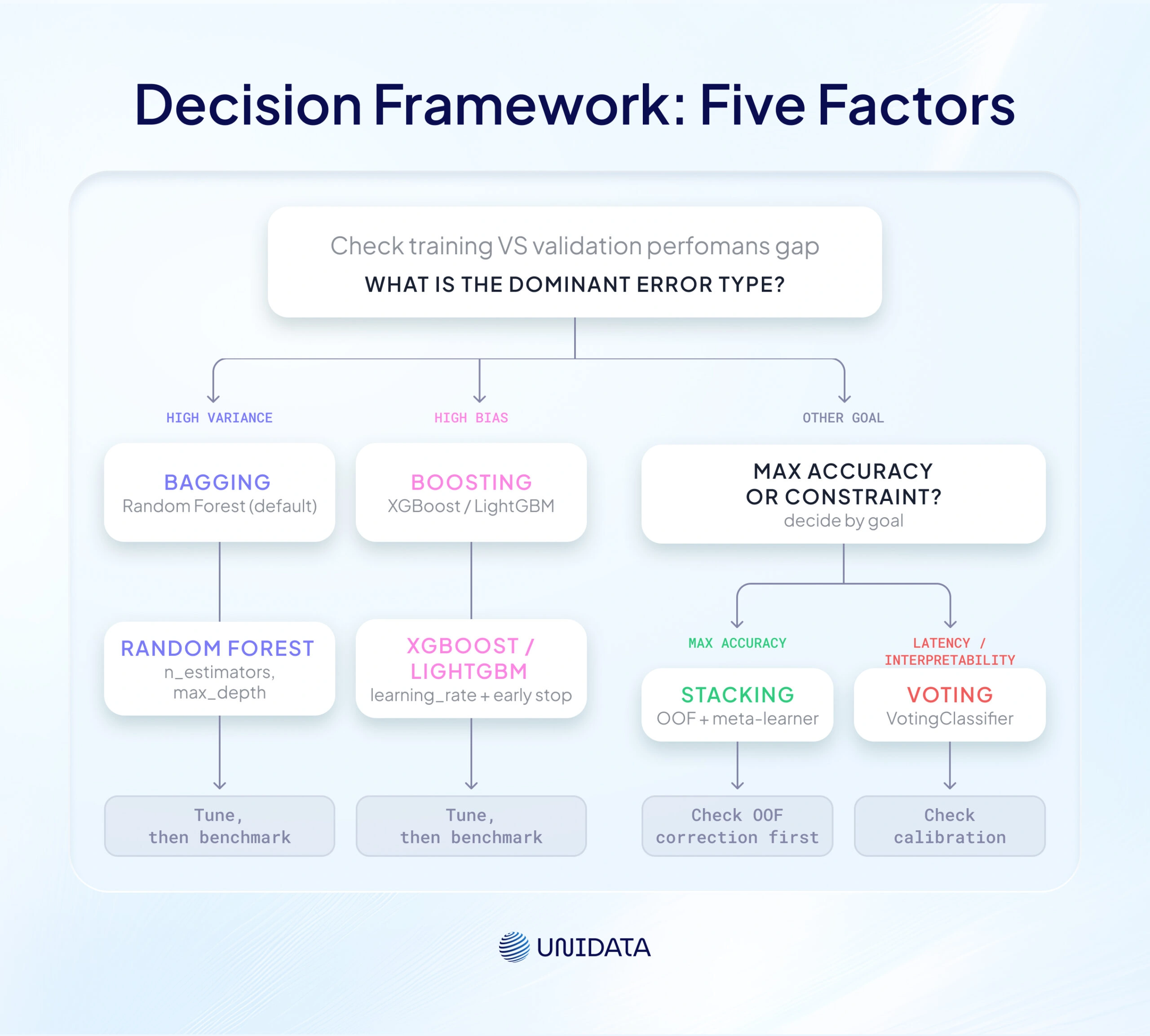
Figure 3: Start with the diagnostic question at the top. If your model changes a lot with small data shifts, that is high variance — go to bagging. If it consistently guesses in the wrong direction, that is high bias — go to boosting. If you need maximum accuracy and have the compute budget, use stacking. If latency or interpretability is a hard constraint, use a simple voting ensemble. Each terminal branch shows the next action.
Ensemble Size — Rules of Thumb
Three Different Rules for Three Different Paradigms
- Random Forest: OOB error plateaus before 300–500 trees. Use oob_score=True to find the plateau cheaply.
- Gradient Boosting (XGBoost / LightGBM): Use early stopping with a validation set. The algorithm determines the optimal round count.
- Stacking: 3–7 diverse base learners is the practitioner consensus. Beyond 7, correlated predictions dominate and signal-to-noise drops.
Tabular Data vs. Deep Learning Ensembles
For structured tabular data, gradient boosted trees and Random Forest remain highly competitive and are often state-of-the-art in practical settings. A 2022 NeurIPS benchmark across 45 datasets found that tree-based models generally outperformed the deep learning approaches evaluated in that study on medium-sized tabular problems. [4]
Deep learning ensembles use distinct strategies for image, text, and audio tasks: snapshot ensembles, multi-start training from different random seeds, and MC-Dropout for uncertainty estimation. [5] These two worlds have largely separate best practices. Choose based on data type, not model preference.
Implementing Ensemble Learning Methods
Getting ensemble learning methods right is mostly about pipeline discipline: preprocessing, tuning order, and avoiding leakage.
Data Preparation: Preprocessing by Base Learner
This is the most commonly overlooked practical detail in ensemble pipeline design.
- Tree-based models (Random Forest, XGBoost, LightGBM) are insensitive to feature scaling and handle missing values natively in modern implementations.
- Linear models and SVMs require scaled inputs and explicit imputation.
- Neural networks require both.
In a stacking pipeline, different base learners need different preprocessing. Use scikit-learn Pipeline objects to encapsulate preprocessing per base learner rather than applying global transformations that compromise some models.
Pseudocode: How the Pipeline Runs
ALGORITHM: Ensemble Learning with Majority Voting
─────────────────────────────────────────────────
INPUT: Training set (X_train, y_train), test set X_test
Base learners: {M1, M2, ..., Mk}

1. FOR each base learner Mi:
a. Train Mi on (X_train, y_train)
b. predictions_i ← Mi.predict(X_test)

2. FOR each test instance x:
a. votes ← {pred_1(x), pred_2(x), ..., pred_k(x)}
b. final_pred(x) ← mode(votes) [classification]
← mean(votes) [regression]

3. RETURN final_predictions
─────────────────────────────────────────────────
Step 1: Each model trains independently on the same dataset.
Step 2a: Each model votes on every test instance.
Step 2b: Majority vote (or mean) is the ensemble's prediction.
Step 3: Output is assembled from combined predictions.
Hyperparameter Tuning — Step by Step
- Tune base learners individually first. A common starting point is Optuna with 100–200 trials per model — Bayesian optimization tends to find good hyperparameters more efficiently than grid search in high-dimensional parameter spaces, though the right trial count depends on your compute budget and search space size.
- Tune the combination strategy second. For stacking, use
GridSearchCVintegrated withStackingClassifierto optimize meta-learner hyperparameters. - Use nested cross-validation to get unbiased performance estimates. Flat CV that reuses the same folds for both base learner tuning and meta-learner training introduces optimistic bias.
For XGBoost and LightGBM, tune these first: learning_rate, n_estimators (via early stopping), max_depth, subsample, and colsample_bytree.
Top 6 Pitfalls — And How to Avoid Them
Top 6 Ensemble Pitfalls
- Meta-learner overfitting — Too few folds (e.g., 2-fold) gives the meta-learner too little OOF data. Use 5–10 folds and a regularized meta-learner (Ridge, constrained LightGBM).
- Data leakage in OOF generation — Training a base learner on fold N and evaluating on fold N inflates predictions. Always validate on held-out folds only.
- Excessive model correlation — Adding 10 XGBoost variants with similar hyperparameters adds noise, not signal. If pairwise OOF correlation exceeds 0.95, drop the redundant model.
- Re-tuning base learners after assembling the stack — This invalidates meta-learner training data. Lock base learners before training the meta-learner.
- Feature preprocessing leakage — Fitting scalers or imputers on the full training set before CV splits leaks statistics across folds. Fit all preprocessing inside the CV loop.
- Diminishing returns ignored — Benchmark every new base learner on a held-out set. Set a minimum improvement threshold in advance (for example, 0.001 AUC) and skip any addition that doesn't clear it. The exact number should reflect what matters for your specific problem.
Evaluating and Interpreting Ensemble Learning Methods
Evaluation is not a technical default — it reflects what failure costs in your specific context. Pick metrics and monitoring signals before you build, not after.
Metric Selection — A Business Decision First
- AUC-ROC — Measures ranking quality. Use when false positive and false negative costs are asymmetric.
- Log-loss — Measures probability calibration quality. Use when downstream decisions depend on predicted probabilities.
- RMSE / MAE — Standard regression metrics. RMSE penalizes large errors more heavily.
- Calibration curves — Reveal whether predicted probabilities match empirical frequencies. Frequently neglected and frequently consequential.
A documented failure mode: a team optimized AUC on a credit scoring model, achieved strong ranking performance, but poorly calibrated probabilities caused the downstream risk system to systematically underestimate default rates. Always track CV stability — standard deviation across folds alongside mean CV score. High fold-to-fold variance signals that the ensemble will not generalize.
Feature Importance — Three Methods, One Clear Ranking
Three approaches exist, and they disagree more often than practitioners expect:
- Mean Decrease Impurity (MDI) — Built into
feature_importances_ in scikit-learn. Fast but biased toward high-cardinality features. Scikit-learn's own documentation flags this limitation explicitly. - Permutation Importance — Measures performance drop when a feature is randomly shuffled. More reliable than MDI; heavier to compute.
- SHAP Values — The current best practice. Provides local (per-prediction) and global explanations based on game-theoretic Shapley values.
For communicating importance to non-technical stakeholders: a ranked bar chart of mean absolute SHAP values is the most reliable and intuitively interpretable format.
Interpretability Tools — SHAP, LIME, and PDPs
Use SHAP as the primary interpretability tool for ensemble models. The SHAP library provides TreeExplainer for Random Forest, XGBoost, and LightGBM - exact Shapley values computed efficiently. Standard production workflow:
- Train the ensemble; generate predictions on a validation set
- Initialize
shap.TreeExplainer(model)and computeshap_values - Use
shap.summary_plot()for global importance;shap.waterfall_plot()for per-prediction local explanations
LIME and Partial Dependence Plots (PDPs) complement SHAP: LIME generates local linear approximations useful when SHAP is unavailable; PDPs show the marginal effect of a feature on predictions and help surface non-linear relationships.
Algorithmic Bias in Ensemble Learning Methods
Ensemble learning methods are not immune to algorithmic bias when trained on historically biased data. A 2019 study in Science found that a widely used healthcare prediction algorithm affecting millions of patients showed significant racial disparity: at the same predicted risk score, Black patients were substantially sicker than White patients. The algorithm's bias originated in its choice of healthcare cost as a proxy for health status — a structural data problem, not a modeling failure. [6]
Practitioners deploying ensemble models in consequential settings should evaluate:
- Demographic parity — Are positive prediction rates equal across demographic groups?
- Equalized odds — Are true positive and false positive rates equal across groups?
Fairness evaluation is not a one-time exercise. Monitor for drift as the data distribution changes over time.
Real-World Applications of Ensemble Learning Methods
The most systematically documented evidence for ensemble learning methods comes from two sources: competition leaderboards and industry deployments. Both tell the same story.
What Kaggle Results Teach Us
Top-finishing solutions in tabular competitions almost universally employ multi-level stacking, with LightGBM and XGBoost appearing as base learners in the majority of top-10 solutions. The Netflix Prize is the clearest example: the winning team blended hundreds of models across multiple stacked layers to take the $1M prize. Ensembling's edge holds even when the underlying problem is brutally hard - academic analysis of the Heritage Health Prize found ensembles consistently beat single models, even though no team's solution was accurate enough to win the competition outright.
The connection to production applicability is direct: the same leakage-prevention, diversity-management, and early-stopping principles that win competitions are the ones that produce robust production models.
Industries Where Ensemble Methods Win
Five Industry Applications with the Preferred Technique
- Fraud Detection — Random Forest and gradient boosting identify anomalous transaction patterns. Ensembles handle class imbalance better than single models and produce calibrated probability scores for fraud scoring systems.
- Healthcare Diagnostics — Ensemble classifiers applied to clinical data and medical imaging (MRI segmentation, disease prognosis from EHR data) outperform single models on rare-disease detection tasks where recall is critical.
- Credit Scoring and Finance — Gradient boosting (XGBoost, LightGBM) dominates credit default prediction and bankruptcy modeling benchmarks. Strong performance on mixed-feature tabular financial data drives widespread adoption.
- Cybersecurity — Ensemble classifiers detect malware and network intrusions with lower false-positive rates than single models. The multi-model structure provides robustness against adversarial feature manipulation.
- Remote Sensing — Bagging and boosting applied to satellite imagery achieve high accuracy on land-cover classification and change-detection tasks where training labels are scarce, and noise is high.
A Recommended Starting Stack for Tabular Classification
The practitioner consensus on a strong default configuration:
- Base learners: LightGBM + XGBoost + CatBoost + Ridge + ExtraTrees
- Meta-learner: Ridge regression (constrained) or LightGBM with strong regularization
- Fold configuration: 5-fold or 10-fold stratified K-fold
The Ridge meta-learner is a deliberate regularization choice. Its L2 penalty prevents the meta-learner from overfitting to idiosyncratic base learner outputs — directly mitigating the first pitfall in the implementation section above. These are commonly used starting points for adaptation, not universal prescriptions.
The Future of Ensemble Learning Methods
Ensemble learning methods are not static. Three active development areas are reshaping how practitioners build and deploy them.
Neural Network Ensembles
The most practically relevant deep ensemble techniques are:
- Deep Ensembles — Training the same architecture from multiple random initializations and averaging predictions. Lakshminarayanan et al. (2017) established this as the standard for calibrated uncertainty estimation in neural networks. [5]
- Snapshot Ensembles — Saving model checkpoints at different points in a cyclical learning rate schedule and averaging predictions at inference time, achieving ensemble diversity at near-zero extra training cost.
- Stochastic Weight Averaging (SWA) — Averaging model weights at different training checkpoints rather than averaging predictions.
- MC-Dropout — Using dropout at inference time to generate multiple stochastic predictions that approximate Bayesian uncertainty estimates.
For structured tabular data, classical gradient boosting ensembles still win. Neural network ensembles add the most value for image, text, audio, and other unstructured data domains. [4]
AutoML — Good for Baselines, Not a Replacement
AutoML frameworks have made ensemble construction accessible without deep manual configuration:
- AutoGluon — Default configuration uses multi-layer stacking and reaches competitive performance with minimal user input.
- Auto-sklearn — Bayesian optimization selects and configures base learners and meta-learners automatically.
- H2O AutoML — Produces stacked ensembles and individual models with automated hyperparameter tuning.
Use AutoML to set a strong baseline quickly. Do not mistake a strong AutoML baseline for a production-ready system — data quality issues, domain-specific feature engineering, and fairness requirements still require human judgment.
Foundation Models and Ensembles — Coexistence
Large language models have reshaped NLP and generative AI. They have not displaced ensemble methods for structured data. The empirical evidence suggests that gradient boosting ensembles remain among the strongest-performing approaches on many tabular benchmarks. [4]
The practical picture going forward is hybrid, not winner-take-all: using foundation model embeddings as features in classical ensemble pipelines, and ensembling fine-tuned LLMs for NLP classification tasks. Mixture-of-Experts architectures within large models are themselves an ensemble principle applied at the parameter level.
Conclusion
Ensemble learning methods work because model diversity is a signal. When models with different failure modes are combined correctly, their noise cancels, and their shared signal amplifies.
The bias–variance tradeoff is the practical guide: high-variance problems call for bagging, high-bias problems call for boosting, and maximum-performance targets with sufficient data justify stacking's added complexity.
Start with the simplest ensemble that addresses your dominant error type. A weighted average benchmarked on a held-out set is more valuable than an elaborate stacking architecture built on assumptions. Add complexity only when the validation set shows it is worth it.
Frequently Asked Questions (FAQ)
Ensemble learning is a machine learning approach that combines predictions from multiple models (base learners) into a single output. By aggregating models with different strengths and weaknesses, ensembles often achieve better accuracy, stability, and generalization than individual models.
The three core ensemble learning methods are:
- Bagging – trains models independently on different bootstrap samples and combines their predictions (e.g., Random Forest).
- Boosting – trains models sequentially, with each model correcting errors made by previous models (e.g., XGBoost, LightGBM, CatBoost).
- Stacking – trains a meta-learner to combine predictions from multiple base models.
Voting and averaging are simpler ensemble techniques that combine model outputs without a learned meta-model.
Bagging and boosting target different sources of prediction error.
- Bagging primarily reduces variance by training independent models in parallel and aggregating their predictions.
- Boosting primarily reduces bias by training models sequentially, with each new model focusing on previous mistakes.
Bagging is easier to parallelize and is generally more robust to noisy data, while boosting often achieves higher predictive performance when properly tuned.
Ensemble learning works by training multiple models and combining their predictions through averaging, voting, or a meta-learner. If the models make partially independent errors, those errors can cancel out, producing predictions that are often more accurate and stable than those of any individual model.
The best method depends on the problem:
- Use bagging when model variance is the main issue.
- Use boosting when the model underfits and exhibits high bias.
- Use stacking when maximizing predictive performance is the primary objective and additional complexity is acceptable.
- Use voting or averaging when you want a simpler and easier-to-maintain solution.
Benchmarking multiple approaches on a validation set is usually the most reliable way to decide.
Advantages:
- Higher predictive accuracy
- Better generalization
- Reduced sensitivity to overfitting in many cases
- Strong performance on structured/tabular data
Limitations:
- Higher computational cost
- Increased implementation complexity
- Reduced interpretability
- Longer training and inference times
Ensembles are not always justified when latency, simplicity, or explainability are critical requirements.
Further Reading & References:
- [1] Breiman, L. — Random Forests — Machine Learning, Vol. 45, pp. 5–32 — 2001
- [2] Freund, Y. & Schapire, R. E. — A Decision-Theoretic Generalization of On-Line Learning and an Application to Boosting — Journal of Computer and System Sciences, Vol. 55, No. 1, pp. 119–139 — 1997
- [3] Chen, T. & Guestrin, C. — XGBoost: A Scalable Tree Boosting System — Proceedings of the 22nd ACM SIGKDD International Conference on Knowledge Discovery and Data Mining, pp. 785–794 — 2016
- [4] Grinsztajn, L., Oyallon, E. & Varoquaux, G. — Why Do Tree-Based Models Still Outperform Deep Learning on Tabular Data? — NeurIPS 2022
- [5] Lakshminarayanan, B., Pritzel, A. & Blundell, C. — Simple and Scalable Predictive Uncertainty Estimation using Deep Ensembles — NeurIPS 2017
- [6] Obermeyer, Z., Powers, B., Vogeli, C. & Mullainathan, S. — Dissecting Racial Bias in an Algorithm Used to Manage the Health of Populations — Science, Vol. 366, No. 6464, pp. 447–453 — 2019