

Introduction
Every machine learning model has one job: to learn something general from specific examples. Not to memorize the training data, and not to oversimplify it — but to find the patterns that actually hold up when new data arrives. Getting this right is harder than it sounds, and when it goes wrong, it goes wrong in one of two predictable ways.
Overfitting happens when a model learns its training data too well, picking up noise and coincidences alongside genuine patterns. It looks excellent on paper, but then struggles the moment it encounters anything slightly different from what it was trained on. Underfitting is the opposite problem, where the model is too simple, or too constrained, to capture what's actually going on in the data. It performs poorly everywhere, including the training set.
Overfitting and underfitting are among the most common causes of poor model performance in production environments [1]. This guide covers both in full: definitions, the bias-variance tradeoff, diagnostic tools, and a complete set of remedies.
Key Takeaways
- Overfitting happens when a model memorizes training data, including noise, and fails to generalize to new examples, producing high training accuracy but poor real-world performance.
- Underfitting happens when a model is too simple to capture the true patterns in data, performing poorly on both training and test data.
- The bias-variance tradeoff is the theoretical lens that explains both problems: overfitting reflects high variance, and underfitting reflects high bias.
- Diagnose before you fix — applying the wrong remedy makes things worse. Learning curves are often one of the most useful first diagnostic tools when investigating model performance problems.
- Multiple proven techniques exist for both problems, from regularization and dropout for overfitting to feature engineering and complexity increases for underfitting.
What Overfitting and Underfitting Actually Mean
Think of a student preparing for an exam. One student memorizes every practice question word-for-word but can’t answer anything phrased differently. Another barely studies and can only answer the most obvious questions. A third understands the material well enough to handle questions they’ve never seen. The first student is overfitting; the second is underfitting; the third has achieved good generalization.
Machine learning models face the same challenge. The real question isn’t whether a model is “too complex” or “too simple” — it’s whether the model has learned the underlying signal in the data. Models that memorize noise instead of meaningful patterns tend to overfit, while models that fail to capture the signal at all tend to underfit. The goal is to find a balance where the model learns genuine relationships and generalizes well to new data.
Defining Overfitting: When a Model Memorizes Instead of Learns
Overfitting occurs when a model learns the training data so precisely, including its noise and outliers, that it performs poorly on new data. A model might achieve 98% training accuracy while test accuracy sits at 61%.
Three root causes drive this:
- Excessive model complexity — too many parameters relative to training data, giving the model capacity to memorize noise
- Insufficient training data — too few examples force the model to fit noise in the gaps
- Training too long — optimizing past the point of good generalization causes the model to chase noise-driven improvements
The Real-World Consequences of Overfitting
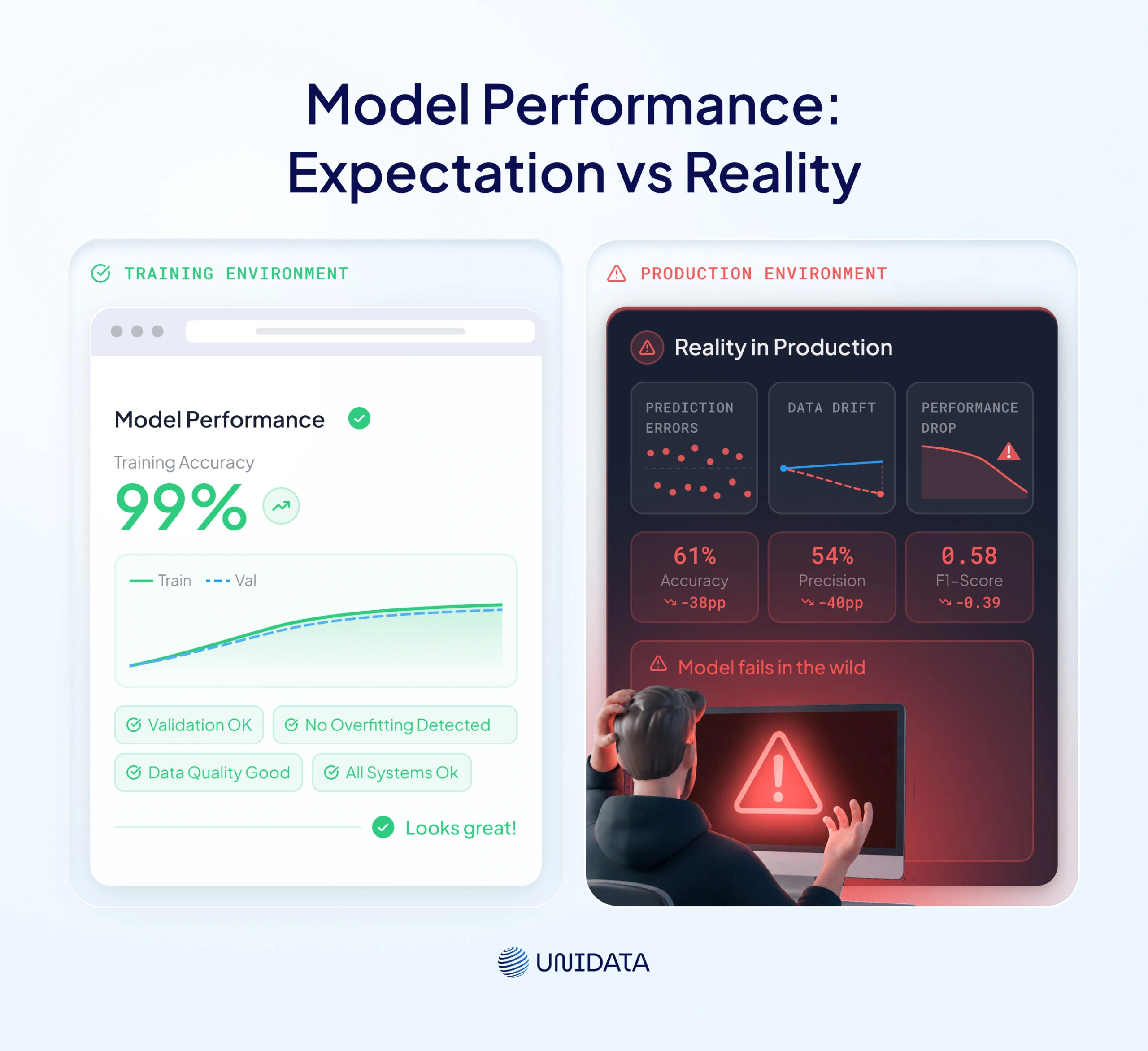
The insidious danger of overfitting is that it creates false confidence. The model appears to work until production reveals otherwise. Specific business costs include:
- Silent production failure — a demand forecasting model overfit to seasonal spikes confidently predicts the wrong inventory levels in slightly different conditions, with no visible error signal until the business impact is already felt
- Erosion of stakeholder trust — once a model collapses in production after strong development metrics, rebuilding confidence with non-technical stakeholders takes far longer than fixing the model itself
- Wasted resources — teams that deploy overfit models often spend months investigating data quality, system infrastructure, and business logic changes before realizing the root cause is the model itself
- Dangerous false positives or negatives — a fraud detection model overfit to historical fraud patterns generates excessive false positives, blocking legitimate customers while failing to catch novel fraud patterns
Defining Underfitting: When a Model Is Too Simple to Be Useful
Underfitting happens when a model fails to capture the underlying patterns in data, producing high error on both training and test sets. Think of an archer who always misses in the same direction: consistent, but wrong.
Primary causes:
- Model too simple — a linear model applied to non-linear data cannot represent the relationships present, regardless of data volume
- Insufficient or poorly engineered features — even a capable model will underfit if input signals don't encode relevant information
- Excessive regularization — over-aggressive L2 penalty suppresses all learning, not just the noisy variety
The Real-World Consequences of Underfitting
Underfitting rarely causes dramatic failures. Instead, it produces consistently weak predictions because the model never learns the underlying relationships in the data. The result is a system that appears stable but delivers limited business value.
- Oversimplified predictions — a customer churn model that predicts most customers will stay may achieve reasonable accuracy in an imbalanced dataset, yet fail to identify the customers who are actually at risk of leaving.
- Missed opportunities and hidden patterns — a pricing model that stays close to average market prices regardless of demand, competition, or seasonality cannot capitalize on premium opportunities or respond effectively to changing conditions.
- Reduced business impact — when a model consistently overlooks meaningful signals, stakeholders may conclude that machine learning offers little value for the problem, even though the real issue is that the model is too simple to capture the available information.
What a Good Fit Looks Like
A well-generalized model achieves low training error and low validation error, with the two values close together. Good fit is a dynamic target defined by data size, problem complexity, and business requirements — not a universal absolute.
Generalization in Machine Learning: The Foundation of Model Performance
Every technique in machine learning ultimately contributes to a central goal: generalization — performing well on data the model has never seen. Generalization is measured through a structured data split:
$$$\text{Training Set} \rightarrow \text{Validation set} \rightarrow \text{Test Set}$$$
- Training Set teaches the model
- Validation Set guides development decisions
- Test Set provides an unbiased final assessment, used exactly once
What Generalization Error Is and How It Is Measured
Generalization error is the error rate a model produces on new, unseen data from the same distribution. It decomposes into three components:
$$$\text{Total Error} = B^2 + V + E$$$
- $$B^2$$ (Bias²) — systematic error caused by overly restrictive assumptions that prevent the model from capturing underlying patterns
- $$V$$(Variance) — sensitivity to fluctuations in the training data, leading the model to learn dataset-specific noise
- $$E$$ (Irreducible Error) — error arising from measurement noise, missing information, and inherent uncertainty in the data-generating process
This three-component decomposition was formalized by Geman et al. [2] and is explained further in Hastie et al. [3]. The irreducible error insight is frequently omitted from introductory tutorials. It sets a hard performance floor: no matter how sophisticated the model becomes, some prediction error will remain due to factors such as measurement noise, incomplete or unobserved features, label uncertainty, and inherent randomness in the underlying process. Understanding this prevents teams from chasing unrealistic performance targets.
Why Generalization Is More Difficult Than It Appears
Training data is a finite, potentially noisy sample of a much larger reality. The model must infer general patterns from incomplete evidence — a process called inductive learning. The relationship between dataset size and model capacity is one of the most useful diagnostics practitioners can consider [4]. As model complexity increases relative to the amount of available data, the risk of overfitting generally rises, especially when regularization and data augmentation are limited. While modern neural networks can often generalize well even with more parameters than training examples, models with very high capacity require additional care to avoid memorizing noise rather than learning meaningful patterns.
The Bias-Variance Tradeoff: The Theoretical Framework Behind Both Problems
The bias-variance tradeoff gives a principled explanation for why both overfitting and underfitting happen, and why fixing one can worsen the other.
The chart above shows how the three error components behave as model complexity increases. Bias² falls steadily as the model gains the capacity to capture real patterns. Variance rises as the model becomes sensitive to the specific training sample it saw. The total error curve forms a U-shape, with its minimum at the point where the combined penalty of bias and variance is lowest. To the left of that point, the model is underfitting; to the right, it is overfitting. The goal of every diagnostic and remediation technique in this article is to find and stay close to that minimum.
What Bias Means in a Machine Learning Model
Bias is the error from approximating a complex problem with a simplified model — systematic mistakes that persist regardless of data volume. A high-bias archer always shoots left; more practice doesn't fix a wrong stance. In practice, high bias arises in linear regression on non-linear data or in shallow decision trees for complex interaction problems.
What Variance Means and Why It Matters
Variance is the model's sensitivity to small changes in training data. A high-variance model produces wildly different predictions when retrained on a slightly different sample. Cross-validation fold variance is the standard deviation of scores across folds and can provide an early indication of model instability and potential overfitting risk. It should be interpreted alongside learning curves and validation performance rather than used in isolation.
How Bias and Variance Combine: Finding the Sweet Spot
The decomposition formula makes the joint minimization challenge explicit:
$$$\text{Total Error} = B^2 + V + E$$$
where $$B$$ represents bias, $$V$$ represents variance, and $$E$$ is the irreducible error. The objective is to minimize $$B^{2} + V$$, since the irreducible component cannot be reduced by model design. Reducing bias by increasing model complexity often increases variance, while simplifying the model typically lowers variance at the cost of higher bias. Beyond the optimal point, additional complexity increases total error because the growth in variance outweighs the reduction in bias. This sweet spot cannot be calculated analytically for most real-world problems and is usually identified empirically through the diagnostic process described in the next section.
How to Diagnose Overfitting and Underfitting in Models
Most ML projects struggle not because teams lack solutions, but because they misidentify the problem. Adding regularization to an underfitting model reduces performance further, while increasing complexity in an overfitting model amplifies the issue. Before applying any remedy, it is also important to rule out data leakage. Leakage occurs when information that would not be available at prediction time accidentally enters the training process, producing overly optimistic validation results. Accurate diagnosis comes first.
Reading Learning Curves: The Primary Diagnostic Tool
A learning curve shows model performance over training, typically plotting training and validation loss across epochs. It can also be constructed against training set size or training time, depending on what aspect of learning dynamics is being analyzed. In practice, it is one of the primary diagnostic tools.
Three patterns identify three states:
Pattern 1 — Underfitting
Both curves plateau at high error. The model isn't learning even the training data. Address model complexity, features, or data quality.
Pattern 2 — Good Fit.
Both curves converge at low error. Training and validation performance are close together — this is the target state.
Pattern 3 — Overfitting.
Training error drops while validation error plateaus or rises. The model is learning the training set specifically, not the underlying pattern. The widening gap is the generalization gap.
Training vs. Validation Error Gap: Interpreting the Numbers
As a working heuristic, if validation accuracy falls consistently below training accuracy as training progresses, treat it as a signal worth investigating. A growing gap is more meaningful than any absolute threshold. Context matters, namely, the same gap carries different implications in medical imaging versus product recommendations.
Key Metrics to Monitor During Training
Track these signals simultaneously, since no single metric fully describes model behavior:
- Training and validation loss — training loss typically decreases as optimization progresses, while validation loss reflects generalization. What matters is not convergence, but the relationship between the two: a widening gap indicates overfitting, while consistently high values on both suggest underfitting.
- Task-specific metric (accuracy, F1, RMSE) — evaluates performance in terms directly aligned with the business objective and is often more interpretable than loss.
- Cross-validation score standard deviation — high variance across folds indicates instability of the model and is itself a signal of poor generalization.
python
from sklearn.model_selection import cross_val_score
from sklearn.ensemble import RandomForestClassifier
import numpy as np

model = RandomForestClassifier(n_estimators=100, random_state=42)
scores = cross_val_score(model, X, y, cv=10, scoring='accuracy')

print(f'Mean accuracy:  {scores.mean():.3f}')
print(f'Std deviation:  {scores.std():.3f}')

if scores.std() > 0.05:
    print('Warning: high variance across folds — check for overfitting.')
Proven Techniques to Fix Overfitting
Model Families Most Prone to Overfitting
- Deep neural networks — enormous parameter counts make these highly prone to memorization [5]. Dropout, early stopping, and augmentation are the primary remedies
- Unpruned decision trees — deep trees can easily overfit when allowed to grow without effective constraints such as max_depth, min_samples_leaf, or pruning.
- High-degree polynomial regression — fits arbitrary curves through training data near feature space edges
Regularization Methods: L1, L2, and Elastic Net
Regularization adds a penalty to the loss function that discourages large coefficients.
- L2 (Ridge) — start here by default. Proportional shrinkage handles correlated features well
- L1 (Lasso) — when many features are likely irrelevant [6]. Drives coefficients to zero — automatic feature selection
- Elastic Net — when both conditions apply. Combines L1 and L2
python
from sklearn.linear_model import Ridge, Lasso, ElasticNet
from sklearn.model_selection import GridSearchCV

ridge_cv = GridSearchCV(Ridge(), {'alpha': [0.001, 0.01, 0.1, 1, 10, 100]}, cv=5, scoring='neg_mean_squared_error')
ridge_cv.fit(X_train, y_train)
print('Best lambda (Ridge):', ridge_cv.best_params_)

lasso_cv = GridSearchCV(Lasso(), {'alpha': [0.001, 0.01, 0.1, 1, 10]}, cv=5, scoring='neg_mean_squared_error')
lasso_cv.fit(X_train, y_train)
print('Best lambda (Lasso):', lasso_cv.best_params_)
Ensemble Methods: How Combining Models Reduces Overfitting
- Bagging (e.g., Random Forest [7]) — bootstrap averaging primarily reduces variance. Strong baseline for most tabular problems
- Boosting (e.g., Gradient Boosting) — primarily reduces bias, but can itself overfit with too many trees or too high a learning rate
Dropout and Early Stopping in Neural Networks
Dropout [8] randomly deactivates neurons during training, preventing co-adaptation. A common starting range is 0.2–0.5 for hidden layers, although the optimal value depends on the architecture, dataset size, and task.
Early stopping halts training when validation loss stops improving. Combine with model checkpointing to restore the best weights.
python
import tensorflow as tf
from tensorflow.keras import layers, callbacks

model = tf.keras.Sequential([
tf.keras.Input(shape=(input_dim,)),
layers.Dense(256, activation='relu'),
layers.Dropout(0.25),
layers.Dense(128, activation='relu'),
layers.Dropout(0.25),
layers.Dense(num_classes, activation='softmax')
])
model.compile(optimizer='adam', loss='categorical_crossentropy', metrics=['accuracy'])

early_stop = callbacks.EarlyStopping(monitor='val_loss', patience=10, restore_best_weights=True)
checkpoint = callbacks.ModelCheckpoint(filepath='best_model.keras', monitor='val_loss', save_best_only=True)

model.fit(X_train, y_train, validation_split=0.2, epochs=200, batch_size=32, callbacks=[early_stop, checkpoint])
Data Augmentation
More real data is always the most robust solution. When collection is impractical, augmentation is used to synthetically expand the training set.
For computer vision tasks, this includes transformations such as rotation, flipping, cropping, and color jittering.
For tabular class imbalance problems, a common approach is SMOTE (Synthetic Minority Over-sampling Technique), which generates synthetic samples of the minority class by interpolating between existing examples in feature space using nearest neighbors.
Augmentation methods are highly domain-specific and are not universally transferable across data types; each modality requires techniques that respect its underlying structure and semantics.
python
from tensorflow.keras.preprocessing.image import ImageDataGenerator

augmentor = ImageDataGenerator(rotation_range=15, horizontal_flip=True, width_shift_range=0.1,
                                height_shift_range=0.1, zoom_range=0.1, fill_mode='nearest')
train_generator = augmentor.flow(X_train, y_train, batch_size=32)
model.fit(train_generator, steps_per_epoch=len(X_train) // 32, epochs=50, validation_data=(X_val, y_val))
Pruning Decision Trees and Managing Ensemble Complexity
Use max_depth, min_samples_leaf, or min_samples_split to control tree complexity and prevent uncontrolled growth. For Gradient Boosting models, the interaction between learning_rate and n_estimators is a key tuning dimension: a lower learning rate generally requires more trees to reach optimal performance. Instead of manually guessing the optimal number of trees, early stopping can be used to terminate training when validation performance stops improving.
from sklearn.ensemble import GradientBoostingClassifier
model = GradientBoostingClassifier(
    learning_rate=0.05,
    n_estimators=500,          # upper bound on number of trees
    max_depth=4,
    subsample=0.8,
    random_state=42,
    validation_fraction=0.1,
    n_iter_no_change=10,
    tol=1e-4
)
model.fit(X_train, y_train)
print(f"Optimal number of trees: {model.n_estimators_}")
Proven Techniques to Fix Underfitting
Underfitting receives far less attention than overfitting, yet it's equally damaging. Teams focused on avoiding overfitting often over-regularize or under-engineer features — and end up with a model that quietly fails to add value.
Model Families Most Prone to Underfitting
- Linear regression / logistic regression — structurally limited to linear decision boundaries. Note: can also overfit when features greatly exceed training examples — "linear = underfitting" is a tendency, not a guarantee.
- Linear discriminant analysis — assumes Gaussian distributions and linear boundaries
Increasing Model Complexity
Add layers, neurons, polynomial features, or switch to a more expressive family. Make incremental changes and check learning curves after each step — large jumps make diagnosis difficult.
Feature Engineering
Underfitting often results from insufficient features, not an inadequate model. High-leverage examples: interaction terms, log transformations for skewed features, cyclical sine/cosine encoding for time-based features.
Removing Noise from Training Data
Heavily noisy or mislabeled data can prevent any coherent signal from being learned, causing underfitting even when the architecture is correct. Run before concluding the model needs to change:
- Outlier detection and investigation
- Missing value imputation review
- Label quality audit on a sample of borderline predictions
Reducing Regularization and Training Longer
If regularization was applied to address overfitting but resulted in poor performance, the regularization strength (λ) may be too high. In such cases, it is appropriate to run a grid search over regularization parameters using cross-validation.
Before making architectural changes, it is important to verify whether the model has actually converged by inspecting the training loss curve. If the training loss is still decreasing, the issue is undertraining rather than true underfitting.
These two conditions can overlap: a model may be both undertrained and ultimately underfit if it lacks sufficient capacity, meaning that even with full convergence it would still fail to capture the underlying signal.
Overfitting vs. Underfitting: Side-by-Side Comparison
The comparison table below distills the core conceptual content of this article into a reference format. The most important rows are the error pattern rows (the diagnostic signature) and the bias/variance levels, which connect the practical observations to the theoretical framework.
| Overfitting | Underfitting | |
|---|---|---|
| Definition | Model memorizes training data including noise | Model too simple to capture data patterns |
| Root cause | High variance — excessive sensitivity to training data | High bias — incorrect model assumptions |
| Training error | Very low | High |
| Test/validation error | High | High |
| Bias level | Low | High |
| Variance level | High | Low |
| Learning curve pattern | Train drops, validation plateaus or rises | Both curves converge at high error |
| Model family examples | Deep neural networks, unpruned trees, high-degree polynomial | Linear regression, logistic regression, shallow trees |
| Primary fixes | Regularization, dropout, early stopping, data augmentation | Add complexity, feature engineering, reduce regularization |
The fundamental difference lies in how the two problems manifest. Overfitting can create a false sense of confidence because the model performs well during development but fails to generalize to new data. Underfitting, by contrast, usually results in poor performance on both training and validation data, making it easier to detect during model development. However, neither failure mode should be considered universally more dangerous. The relative risk depends on the application, the cost of prediction errors, and how model performance is monitored after deployment.
Which Problem Is More Dangerous in Production?
There is no universal answer to whether overfitting or underfitting is more dangerous in production. The severity of either problem depends on the business context, the consequences of prediction errors, and the safeguards surrounding model deployment.
Overfitting is often viewed as particularly problematic because strong development metrics may create unwarranted confidence in a model that does not generalize well to new data. As a result, performance issues may only become apparent after deployment, potentially leading to operational, financial, or reputational costs.
Underfitting, on the other hand, is typically easier to identify because it produces poor results on both training and validation data. However, this does not make it harmless. A severely underfit model can still cause substantial damage if its predictions are used to support important business or operational decisions.
In practice, both problems represent failures of generalization. The goal is not simply to avoid overfitting or underfitting individually, but to achieve a level of model complexity that balances bias and variance appropriately for the problem at hand.
In safety-critical applications, such as medical diagnosis, fraud detection, and autonomous vehicle systems, both overfitting and underfitting can create serious risks. Overfitting may lead to unjustified confidence in a model that performs poorly on real-world data, while underfitting may result in consistently inaccurate predictions that fail to capture important patterns. In either case, the consequences can be severe, which is why rigorous validation, monitoring, and ongoing model evaluation are essential in these domains.
A Practical Workflow for Avoiding Overfitting and Underfitting
Having a structured process is what separates systematic practitioners from those constantly firefighting. The following workflow applies to many supervised machine learning projects and provides a practical starting framework for model development and evaluation. Specific procedures may vary depending on the domain, learning paradigm, deployment environment, and business requirements.
Step-by-Step Model Evaluation Process
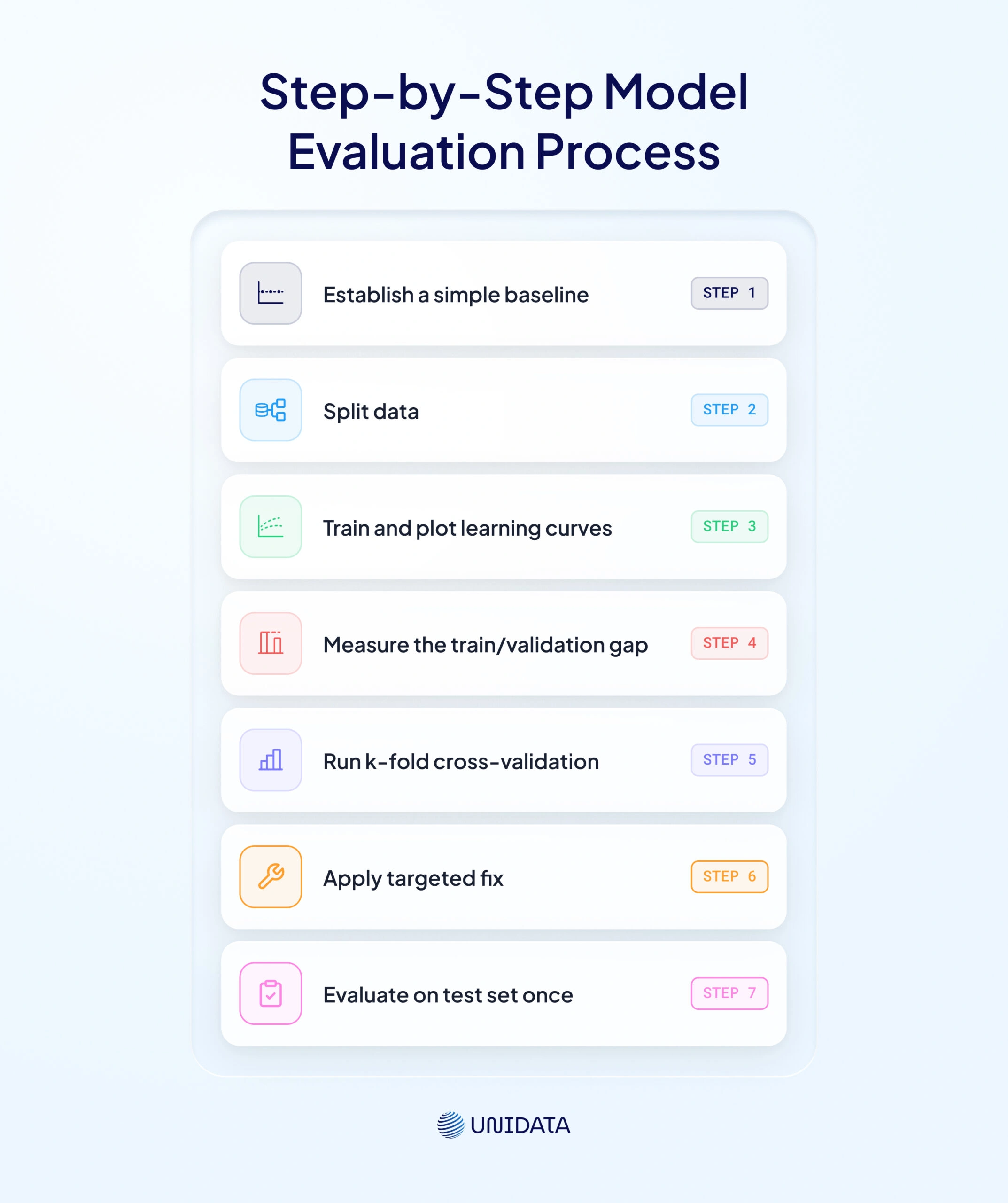
- Establish a simple baseline — defines what underfitting looks like for this specific problem.
- Split data — training, validation, and test sets; hold out the test set until final evaluation.
- Train and plot learning curves — interpret using the three-pattern framework above.
- Measure the train/validation gap — investigate persistent or widening differences between training and validation performance, particularly when validation performance stops improving or begins to deteriorate.
- Run k-fold cross-validation — verify that performance remains consistent across different data splits and assess the stability of the model.
- Apply targeted fix — based on diagnosis, not guessing.
- Evaluate on test set once — after all development decisions are finalized.
Choosing the Right Model Complexity From the Start
A practical starting heuristic: start simple and add complexity only when data demands it. A rough framework:
- Small to moderately sized tabular datasets often benefit from regularized linear models or shallow tree-based methods as strong baselines.
- Larger structured tabular datasets are frequently well served by gradient boosting approaches such as LightGBM or XGBoost.
- Images, text, audio, and other unstructured data are commonly addressed with deep learning models, although the amount of data required depends heavily on the task, model architecture, and availability of transfer learning.
Present this as a starting point, not a hard rule. The learning curve check is always the ultimate arbiter, telling you whether the model you chose is appropriate for your data, regardless of what the heuristic suggested.
Iterative Refinement: The Diagnostic-Fix Loop
Machine learning model development is inherently iterative:
$$$\text{Diagnose} \rightarrow \text{Fix} \rightarrow \text{Evaluate} \rightarrow \text{Diagnose} \rightarrow \text{Fix} \rightarrow \text{Evaluate} \rightarrow \cdots$$$
This is not a sign that something went wrong. It is the nature of the discipline. The inputs to the problem are data, model architecture, hyperparameters, and features that have complex interactions that cannot be fully predicted analytically. Experimentation is the method.
The differentiator between experienced and inexperienced practitioners is often the efficiency of the diagnostic-fix loop. Experienced practitioners tend to formulate better hypotheses, identify likely causes more quickly, and converge on effective solutions with fewer iterations.
Conclusion
Overfitting and underfitting are not isolated problems but two manifestations of the same challenge: achieving reliable generalization. An overfit model learns patterns that do not extend beyond the training data, while an underfit model fails to learn the underlying signal at all. Although their causes and symptoms differ, both ultimately reduce a model's ability to make accurate predictions on unseen data.
The bias-variance tradeoff provides the theoretical framework for understanding these failure modes, but successful model development depends on practical diagnosis rather than theory alone. Learning curves, validation performance, cross-validation, and error analysis help reveal whether a model is suffering from excessive complexity, insufficient capacity, poor features, or limitations in the data itself.
There is no universal model architecture, hyperparameter setting, or workflow that guarantees good performance. Effective machine learning is an iterative process of hypothesis, evaluation, and refinement. The objective is not to maximize training accuracy or minimize a single metric, but to build models that perform consistently, robustly, and reliably when faced with new data.
Ultimately, the most successful practitioners are not those who avoid overfitting or underfitting entirely, but those who recognize these problems early, diagnose them accurately, and apply targeted solutions to improve generalization.
- AI Training
- Robotics
- Data Annotation
- Python
- AWS

Frequently Asked Questions (FAQ)
Overfitting performs well on training data but poorly on new data, because it memorizes noise rather than learning patterns.
Underfitting performs poorly everywhere because it never learned the signal.
Both cause poor generalization through opposite mechanisms.
Plot learning curves. Both converge at high error = underfitting. Training loss dropping while validation rises = overfitting. Confirm with the train/validation gap and k-fold cross-validation score variance.
For neural networks: dropout, early stopping, and augmentation.
For trees: depth limits and Random Forest.
Across all models: L2 regularization as a default and feature selection to remove noisy inputs.
Expected prediction error can be viewed as the sum of three components: bias², variance, and irreducible error. Increasing model complexity often reduces bias but increases variance, while simplifying the model typically has the opposite effect. The goal is to balance these components to achieve the best generalization performance.
Increase model complexity, engineer better features, reduce excessive regularization, clean training data, and verify the model has actually converged before making architectural changes.
Small datasets increase overfitting risk — the model memorizes rather than generalizes. The relevant ratio is data volume to parameter count. Underfitting is less sensitive to dataset size; it’s primarily driven by architecture and feature quality.
The answer depends on the application. Overfitting is often viewed as particularly dangerous because strong development metrics may create unwarranted confidence in a model that fails to generalize after deployment. However, severely underfit models can also cause significant harm if their predictions are used to support important decisions.
Low error on both training and validation sets, with the two values close together. Achieved iteratively through the diagnose-fix-evaluate loop.
Further Reading & References:
- Ying, X. (2019). An Overview of Overfitting and its Solutions. Journal of Physics: Conference Series, 1168, 022022. — A survey covering overfitting causes and remediation techniques across model families.
- Geman, S., Bienenstock, E., & Doursat, R. (1992). Neural Networks and the Bias/Variance Dilemma. Neural Computation, 4(1), 1–58. — The foundational paper that formalized the bias-variance tradeoff.
- Hastie, T., Tibshirani, R., & Friedman, J. (2009). The Elements of Statistical Learning. Springer. — The definitive reference on bias-variance decomposition and regularization theory.
- Domingos, P. (2012). A Few Useful Things to Know About Machine Learning. Communications of the ACM, 55(10), 78–87. — A practitioner-oriented overview of generalization, overfitting, and the curse of dimensionality.
- Goodfellow, I., Bengio, Y., & Courville, A. (2016). Deep Learning. MIT Press. — Chapter 5 covers generalization, capacity, and regularization in depth.
- Tibshirani, R. (1996). Regression Shrinkage and Selection via the Lasso. Journal of the Royal Statistical Society: Series B (Methodological), 58(1), 267–288. — The original paper introducing L1 regularization.
- Breiman, L. (2001). Random Forests. Machine Learning, 45, 5–32. — The foundational Random Forest paper, covering bagging and variance reduction.
- Srivastava, N., Hinton, G., Krizhevsky, A., Sutskever, I., & Salakhutdinov, R. (2014). Dropout: A Simple Way to Prevent Neural Networks from Overfitting. Journal of Machine Learning Research, 15(1), 1929–1958.