

Markov models have historically been used in applications such as autocomplete, spam filtering, recommendation systems, speech recognition, and web search. Although many modern systems now incorporate deep learning, Markov models remain widely used because their transition probabilities are explicit and interpretable, making them easier to audit and validate than many black-box alternatives.
This guide covers six widely used Markovian modeling frameworks, the mathematics behind them, real-world applications, and a step-by-step Python implementation.
What Is a Markov Model?
A Markov model is a probabilistic framework used to describe systems that transition between states over time, where the probability of the next state depends on the current state under a simplifying assumption of limited memory. In practice, this assumption is often an approximation rather than a strict property of the underlying real-world system.
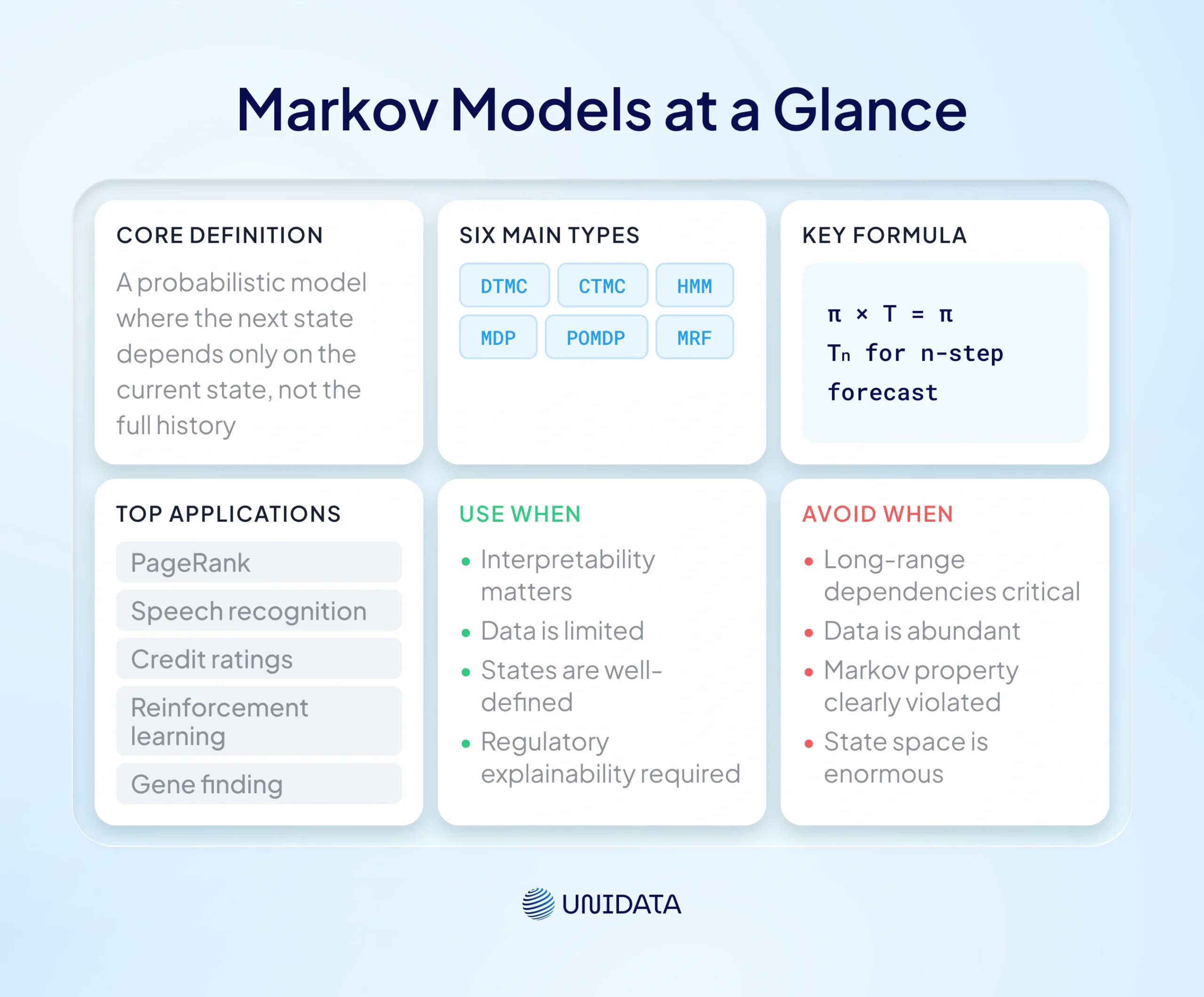
In simplified models such as weather forecasting, the probability of tomorrow’s weather is assumed to depend only on today’s conditions. Real atmospheric systems are far more complex, but the Markov assumption can still provide a useful and tractable approximation.
Russian mathematician Andrey Markov developed the mathematical foundations of Markov chains in the early twentieth century, beginning with studies of letter sequences in literary texts. His framework gave probability theory a new tool: a way to model sequences where the past informs the future through the present, rather than through an infinite accumulation of history.
Every Markov model rests on four components:
- State space — the full set of conditions the system can be in (e.g., Sunny, Cloudy, Rainy)
- Transition probabilities — the probability of moving from any one state to any other
- Initial state distribution — the probability of starting in each state
- Time index — discrete (daily steps) or continuous (events can happen at any moment)
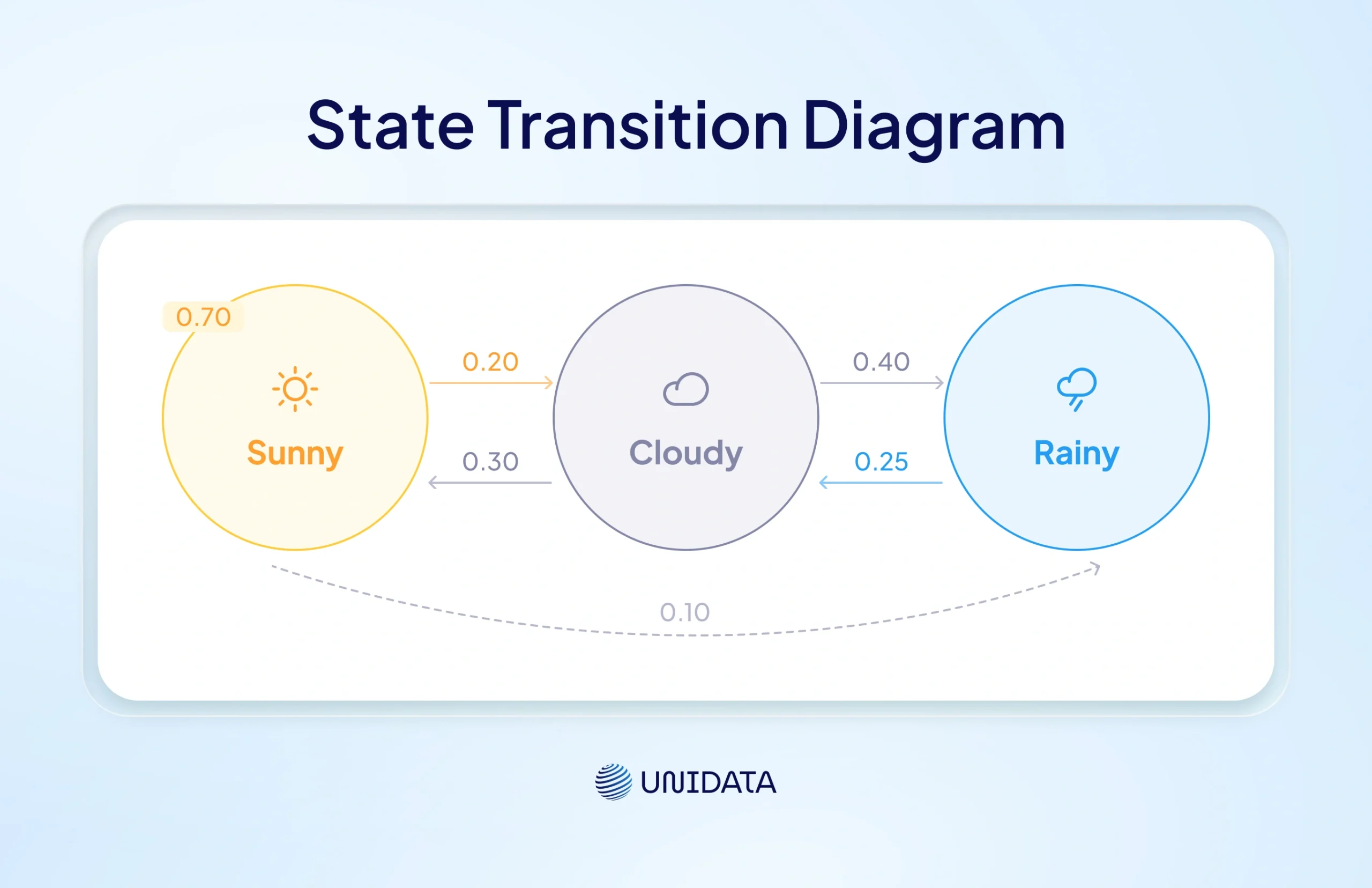
Three-state weather Markov chain. Each arrow shows the probability of transitioning to another state. All outgoing probabilities from any node sum to 1.
The Markov Property and Memorylessness
The defining characteristic of classical Markov models is the Markov property. Formally:
$$$ P(X_{t+1}=x \mid X_t, X_{t-1}, \ldots, X_0)=P(X_{t+1}=x \mid X_t)$$$
In plain English: the probability of being in state x tomorrow depends only on which state you are in today, not on the entire sequence of states you passed through to get here. Today’s state is assumed to encode all the relevant information about the future.
A common misconception is that the term 'memoryless' implies that the model ignores context. It does not. It means the current state is rich enough to capture everything that matters. In some disease progression models, states are defined broadly enough to summarize clinically relevant information from earlier stages. Whether the Markov assumption is reasonable depends on how well the state representation captures the factors that influence future outcomes.
Markov Model Assumptions
Before relying on a Markov model’s outputs, it is important to assess how well the modeling assumptions align with the data and whether deviations are acceptable for the task.
- Mutual exclusivity: each observation must belong to exactly one state. Violations lead to ambiguous state assignment and invalid transition estimates.
- Collective exhaustiveness: the state space should cover all relevant system conditions. Missing states bias transition probabilities by forcing unmodeled outcomes into existing categories.
- Time-homogeneous transitions: transition probabilities are assumed constant over time. If they vary, a non-stationary or time-inhomogeneous model may be more appropriate.
- First-order (Markov) assumption: the next state depends only on the current state. If longer history improves prediction, higher-order models or alternative sequence models may be needed.
A History of Markov Models
The development of Markov models reflects a steady expansion from theoretical probability into a general framework for sequential decision-making and stochastic systems. What began as an abstract study of dependent random variables evolved into a foundational tool across physics, computer science, and artificial intelligence.
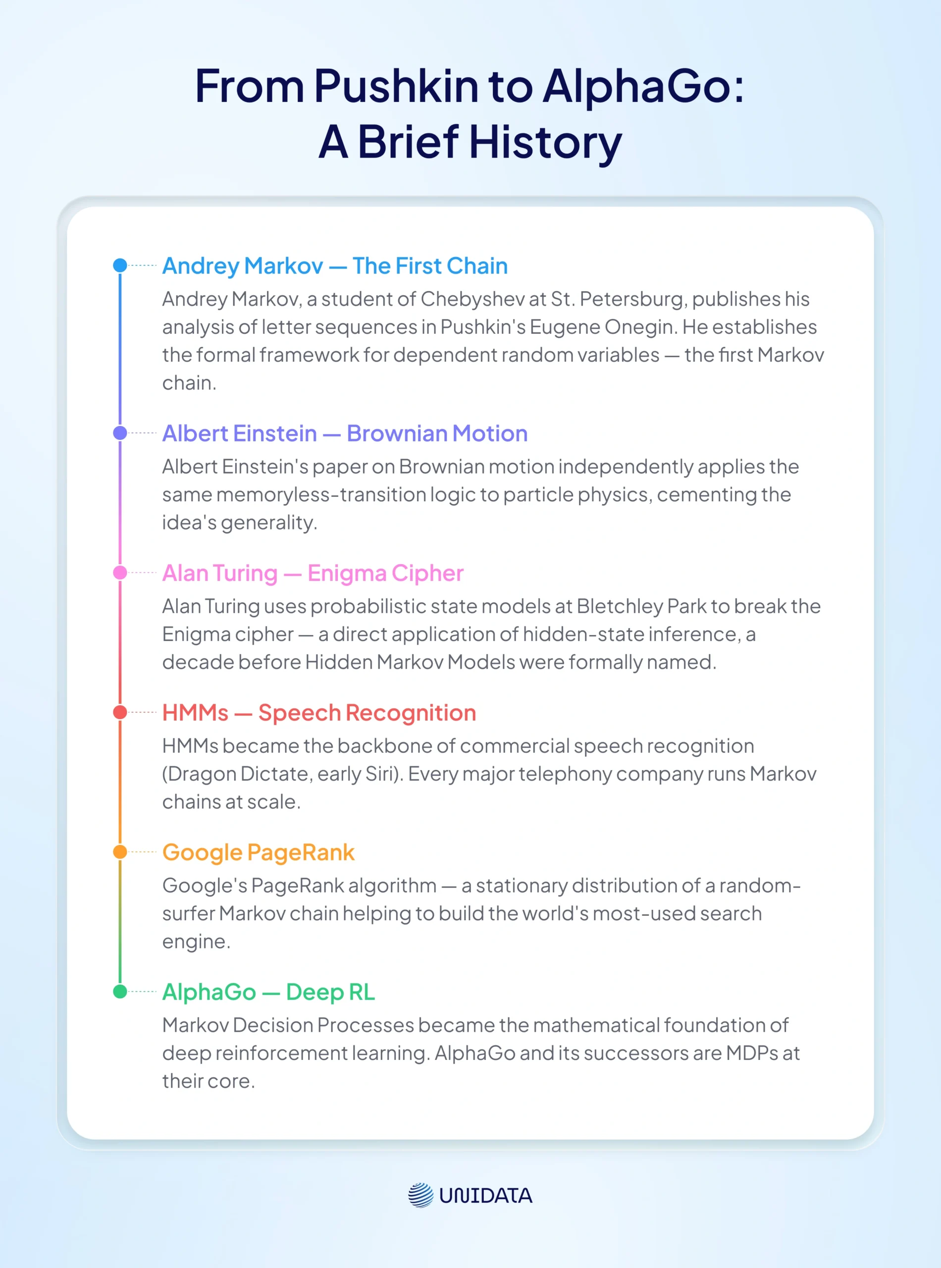
Across these developments, the core idea remains consistent: complex systems can be modeled as transitions between states governed by probabilistic rules.
Types of Markov Models — Choosing the Right Framework
Selecting an inappropriate Markov model variant can lead to misleading results and incorrect assumptions about the underlying process. The comparison table below provides a high-level overview of the major Markov model variants.
| Model | Time | States Observable? | Agent Controlled? | Best Used For |
|---|---|---|---|---|
| DTMC | Discrete | Yes | No | Text prediction, customer churn, board games |
| CTMC | Continuous | Yes | No | Queuing systems, epidemics, chemical kinetics |
| HMM | Discrete | No (hidden) | No | Speech recognition, POS tagging, gesture detection |
| MDP | Discrete | Yes | Yes | Robotics, game AI, recommendation engines |
| POMDP | Discrete | Partially observable | Yes | Autonomous vehicles, medical treatment planning |
| MRF | Spatial | Yes | No | Image segmentation, spatial statistics |
All six types share a 2×2 organizing logic: autonomous (the system evolves on its own) vs. controlled (an agent takes actions), and fully observable (you can see the current state) vs. partially observable (you cannot). DTMCs and CTMCs sit in the autonomous/observable cell. HMMs shift to autonomous/hidden. MDPs add an agent with full observability; POMDPs add an agent facing hidden states.
Discrete-Time Markov Chains (DTMC)
The DTMC is the foundational form. State transitions happen at fixed time steps — day to day, transaction to transaction — governed by a constant transition matrix. Using the weather example, the 3×3 transition matrix looks like this:
T =
| → | Sunny | Cloudy | Rainy |
|---|---|---|---|
| Sunny | 0.70 | 0.20 | 0.10 |
| Cloudy | 0.30 | 0.30 | 0.40 |
| Rainy | 0.10 | 0.25 | 0.65 |
Weather example transition matrix. Each row sums to 1.0 — the system must always transition to some state, including staying in the current one.
Continuous-Time Markov Chains (CTMC)
CTMCs drop the fixed time-step assumption — transitions can happen at any moment, not just at discrete intervals. Instead of a transition matrix, the model uses a rate matrix (Q-matrix) that captures how quickly the system moves between states. Waiting times between transitions follow an exponential distribution.
A CTMC is defined by a generator matrix (or Q-matrix) $$Q=[q_{ij}]$$, where each off-diagonal entry $$q_{ij}$$ represents the instantaneous transition rate from state $$i$$ to state $$j$$. The diagonal elements are defined so that each row sums to zero:
$$$q_{ii}=-\sum_{j\neq i} q_{ij}$$$
This property ensures that $$Q$$ is a valid generator matrix for a continuous-time Markov process. The practical difference from a DTMC is significant: a hospital's patient flow system doesn't admit and discharge patients on a fixed schedule — events happen continuously. CTMCs model this naturally. Other common applications include call center queuing, server load balancing, and epidemic spread modeling, where event timing matters as much as the transitions themselves.
Hidden Markov Models (HMM)
In an HMM, the true state of the system is hidden. What you observe are indirect signals — "emissions" — that carry probabilistic information about the underlying state. A classic example is emotional state recognition, where the true emotional state is hidden and only observable through indirect signals such as speech, facial expressions, or behavior.
Formally, an HMM consists of hidden states $$X_t$$ and observations $$O_t$$. Emission probabilities govern the observation process:
$$$b_j(o_t) = P(O_t = o_t \mid X_t = j)$$$
which specify the probability of observing $$o_t$$ when the hidden state is $$j$$.
Three canonical HMM problems drive most applications:
- Evaluation (Forward Algorithm) — given a sequence of observations, how likely is it under this model?
- Decoding (Viterbi Algorithm) — what is the most likely hidden state sequence that produced these observations?
- Learning (Baum-Welch Algorithm) — given observations, learn the transition and emission probabilities.
The joint probability of a hidden-state sequence and an observation sequence can be expressed as:
$$$P(X_{1:T}, O_{1:T})=P(X_1)\prod_{t=2}^{T} P(X_t \mid X_{t-1})\prod_{t=1}^{T} P(O_t \mid X_t)$$$
This factorization combines transition probabilities between hidden states with emission probabilities linking hidden states to observed data.
Before the widespread adoption of deep neural networks, HMMs were the dominant framework for commercial speech recognition systems. They are still used for part-of-speech tagging, biological sequence analysis, and any resource-constrained system where an LSTM is too expensive to run. HMMs remain an important probabilistic modeling framework in speech processing, bioinformatics, sequence labeling, and other domains where interpretable sequential inference is valuable. [1]
Markov Decision Processes (MDP)
An MDP extends a Markov chain by incorporating actions and rewards and serves as a foundational framework for reinforcement learning. MDPs are commonly defined as (S, A, T, R, γ), where γ is the discount factor.
Imagine a robot navigating a warehouse. At each step, it chooses an action (move left, move right, pick up item). The environment responds with a new state and a reward signal. The robot's goal is to learn a policy — a mapping from states to actions — that maximizes total expected reward over time. The Bellman equation provides the recursive framework used to evaluate and optimize decision-making policies. [5]
A Deep Dive into AI Model Training: Concepts, Techniques, and Best Practices
Learn more
Many reinforcement learning systems, including AlphaGo, are formulated using the Markov Decision Process framework, although practical implementations often incorporate neural networks to handle large state spaces.
Deep learning adds function approximation for large state spaces, but the MDP framework is unchanged from what Bellman described in 1957.
Partially Observable MDPs (POMDP)
POMDPs combine the hidden-state structure of HMMs with the agent-action structure of MDPs. When a robot vacuum cannot see through walls, it maintains a belief state — a probability distribution over all possible current locations — and takes actions to minimize uncertainty while completing its task. The computational cost of solving POMDPs grows rapidly as state and observation spaces expand. Because exact solutions are generally computationally intractable, practical applications rely heavily on approximation methods and heuristic planning techniques.
Markov Random Fields (MRF)
MRFs extend the Markov concept from time to space. Instead of asking "what comes next in a sequence?", an MRF asks "what does my neighbour look like?" Each variable depends only on its immediate spatial neighbours, not on the full field. This makes MRFs the natural tool for problems where dependencies are defined by proximity rather than order. Although Markov Random Fields share the Markov property, they are generally classified as probabilistic graphical models rather than temporal Markov chains. Instead of modeling transitions through time, they model dependencies across neighboring variables in a graph or spatial structure.
The canonical application is image segmentation: each pixel's label (sky, ground, object) depends on the labels of surrounding pixels. MRFs are also used in social network analysis, spatial statistics, and any domain where the data lives on a graph rather than a timeline. Advanced readers will recognize MRFs as a gateway into the broader probabilistic graphical model literature.
The Mathematics Behind Markov Models
Several mathematical concepts form the foundation of practical Markov model analysis and interpretation. You do not need to derive them from scratch — understanding what each one does is enough to build and interpret models responsibly.
The Transition Matrix
The transition matrix T is the central mathematical component of a discrete-time Markov model. Entry T[i][j] gives the probability of moving from state i to state j in one step. Every row must sum to 1.0 because the system must end up somewhere after each step — this is called the row-stochastic property.
To compute the probability distribution n steps into the future, raise the matrix to the power n:
$$$\pi_n=\pi_0 T^n$$$
where $$\pi_0$$ is the initial state distribution vector. This matrix exponentiation is precisely what numpy.linalg.matrix_power(T,n) computes.
Stationary Distribution
The stationary (steady-state) distribution π is the long-run probability vector: the fraction of time the chain spends in each state as time goes to infinity. It satisfies:
$$$\pi \times T=\pi,\quad\sum_i\pi_i=1$$$
- where $$π$$is treated as a row vector
For illustration, a stationary distribution might be $$π$$ = [0.50, 0.25, 0.25], meaning 50% of days are sunny in the long run, regardless of today’s weather. This is precisely the principle underlying Google’s PageRank, which computes the stationary distribution of a random web-surfer Markov chain.
A unique stationary distribution exists when the chain is ergodic — both irreducible (all states are reachable from each other) and aperiodic (no fixed cycle length).
The Chapman-Kolmogorov Equation
The Chapman-Kolmogorov equation provides the formal basis for multi-step predictions:
$$$T^{(m+n)} = T^{m} T^{n}$$$
Conceptually, the probability of going from state $$i$$ to state $$j$$ in m+n steps equals the sum over all possible intermediate states of the m-step and n-step probabilities. Practitioners invoke this equation every time they raise a transition matrix to a power — it is the justification for using $$T^{n}$$ as a forecasting tool.
This chart visualizes how a Markov chain evolves and converges toward its long-run behavior.
Starting from an initial state where the system is fully in the “Rainy” state (P(Sunny) = 0 at step 0), the curve shows how the probability of being in the Sunny state changes as the transition matrix is repeatedly applied. At each step, the state distribution is updated using matrix multiplication, reflecting the cumulative effect of repeated transitions.
Over time, the probability of being in the Sunny state stabilizes and converges toward approximately 0.50, which represents the steady-state (stationary distribution) of the system. This is also shown by the horizontal dashed line, which marks the equilibrium probability.
The key insight illustrated by the chart is that, regardless of the initial condition, a regular Markov chain tends to "forget" its starting state and converge to a stable distribution determined only by the transition probabilities. In this example, convergence occurs around step 10–12, after which further iterations produce negligible change.
This behavior demonstrates the core property of ergodic Markov chains: long-term predictions become independent of the initial state and depend only on the transition structure of the system.
Real-World Applications of Markov Models
Natural Language Processing and Text Generation
Before GPT, Markov chains were the dominant language modeling approach. A word-level DTMC assigns a probability distribution over the next word given the current one: given "the cat sat on the ___", the chain scores "mat" higher than "democracy" based on observed transition frequencies.
HMMs remain relevant for part-of-speech tagging, where the hidden state is a grammatical category (noun, verb, adjective) and the observation is the visible word. On constrained devices — think keyboard autocomplete on low-end phones — Markov language models still run in production because they are orders of magnitude cheaper than transformer-based alternatives.
Finance and Market Modeling
Credit rating agencies, including Moody's and S&P, use Markov chains to model rating transitions: a bond rated AAA today has some probability of being downgraded to AA, A, or BBB over the next year. These transition matrices are estimated from historical default data and published in annual reports.
HMMs model hidden market regimes — Bull, Bear, and Sideways — from observable price and volume data. The model infers the most likely hidden regime sequence given observed returns, letting risk managers adjust positioning accordingly. A critical caveat: financial time series frequently violate the stationarity assumption, making Markov finance models pragmatic approximations rather than exact descriptions. This is not a reason to dismiss them; it is a reason to validate them carefully.
Google PageRank — A Markov Chain in Disguise
A random surfer clicks links indefinitely at random. The probability of landing on any given page, in the long run, is that page's PageRank score. Formally, the web graph is represented as a stochastic matrix — each row represents a page, each column a possible destination, with entries set to 1/k for pages with k outgoing links. The surfer's long-run distribution is the stationary distribution of this matrix.
The "damping factor" (typically 0.85) handles dangling nodes and ensures the chain remains ergodic, guaranteeing a unique stationary distribution exists. This formulation became a core component of Google’s original PageRank algorithm, demonstrating how the stationary distribution of a Markov chain could be used to rank webpages according to link structure. PageRank is widely regarded as one of the most influential practical applications of Markov chains in computer science. [4]
Healthcare and Bioinformatics
Disease progression modeling uses Markov chains directly: Healthy → Pre-diabetic → Diabetic → Complications, with estimated transition probabilities derived from clinical cohort data. These models answer questions like "what fraction of pre-diabetic patients will develop complications within five years?" — exactly the kind of long-run population inference the stationary distribution is designed to provide.
In bioinformatics, HMMs detect CpG islands in DNA sequences. The hidden states are "in a CpG island" vs. "not in a CpG island"; the observations are the four DNA bases (A, T, C, G) with different emission probabilities depending on the hidden state. HMM-based gene prediction methods remain foundational in computational biology. [2]
How to Build a Markov Model — Step-by-Step in Python
Here is a practical five-step workflow using Python and NumPy. The full pipeline — from raw sequence data to Monte Carlo simulation — takes fewer than 40 lines of code.
Step 1 — Define the state space.
Identify mutually exclusive, collectively exhaustive states. For a customer lifecycle model: Prospect, Active, At-Risk, Churned, Reactivated. The key design trade-off: too few states oversimplifies; too many creates data sparsity for rare transitions. Start with the minimum number of states that capture the distinctions relevant to your decision.
Step 2 — Estimate the transition matrix from data.
The following function counts observed state-to-state transitions, applies Laplace smoothing to avoid zero probabilities, and converts the counts into a row-stochastic transition matrix whose rows sum to one.
import numpy as np

def estimate_transition_matrix(sequences, n_states, alpha=1.0):
counts = np.zeros((n_states, n_states), dtype=float)

for seq in sequences:
for i in range(len(seq) - 1):
counts[seq[i], seq[i + 1]] += 1

# Laplace smoothing
counts += alpha

row_sums = counts.sum(axis=1, keepdims=True)

return counts / row_sums

# Example: 3-state weather
# 0 = Sunny, 1 = Cloudy, 2 = Rainy

weather_sequences = [
[0, 0, 1, 2, 2, 1],
[1, 1, 2, 0, 0, 1],
[2, 2, 1, 0, 1, 1]
]

T = estimate_transition_matrix(weather_sequences, n_states=3)

print("Transition matrix:")
print(T)
Step 3 — Validate the model.
Before deployment, assess whether a first-order Markov assumption is reasonable for your data. One common approach is to compare first-order and higher-order transition models using likelihood-ratio tests, chi-square-based methods, or out-of-sample predictive performance. If incorporating additional historical states significantly improves prediction accuracy, a simple first-order Markov model may be inadequate. This validation step is often overlooked, even though violations of the Markov assumption can substantially affect model quality. A model that violates the assumption is not necessarily unusable, but its outputs should be interpreted with appropriate caution.
Step 4 — Run simulations and generate predictions.
import numpy as np
def simulate_markov(T, start_state, n_steps, n_sims=1000):
    n_states = T.shape[0]
    final_states = np.zeros(n_states)
    for _ in range(n_sims):
        state = start_state
        for _ in range(n_steps):
            state = np.random.choice(n_states, p=T[state])
        final_states[state] += 1
    return final_states / n_sims
def n_step_distribution(pi0, T, n):
    return pi0 @ np.linalg.matrix_power(T, n)
def stationary_distribution(T):
    eigvals, eigvecs = np.linalg.eig(T.T)
    idx = np.argmin(np.abs(eigvals - 1))
    pi = np.real(eigvecs[:, idx])
    return pi / pi.sum()
This approach assumes the Markov chain has a unique stationary distribution. For finite chains, this is guaranteed when the chain is ergodic (irreducible and aperiodic). Non-ergodic chains may have multiple stationary distributions or may not converge to a single long-run distribution.
Step 5 — Interpret and communicate results.
Remember that every Markov model output is a probability distribution, not a point prediction. The stationary distribution answers strategic "what happens in the long run?" questions. N-step distributions answer tactical "what is the probability of being in state X in three months?" questions. Always report confidence intervals around transition probability estimates, especially when training data is sparse.
Markov Model vs. Other Predictive Models
Model selection is a context-dependent decision, not a ranking. The right question is not "which model is best?" but "which model best fits the constraints of this problem?"
| Criterion | Markov Model | LSTM / Transformer | Bayesian Network |
|---|---|---|---|
| Interpretability | High — explicit transition probabilities | Low — black box weights | High — explicit conditional dependencies |
| Data requirements | Low to medium | High | Medium |
| Computational cost | Low — matrix operations | High — GPU-intensive | Medium |
| Long-range dependencies | Limited (first-order) | Strong | Explicit (graph structure) |
| Handles non-stationarity | Poorly (time-inhomogeneous extension needed) | Yes | Partially |
| Best use case | Regulated domains, constrained hardware, well-defined states | Complex sequential patterns, large data | Multi-variable causal reasoning |
In banking, healthcare, and insurance, the Markov model's interpretability advantage is not just a nice-to-have — it is often a regulatory requirement. A credit-scoring model that cannot explain why a customer was denied a loan may face additional compliance, transparency, and governance requirements under regulations such as the EU AI Act. In regulated industries such as healthcare, banking, and insurance, explainability, documentation, and auditability requirements may influence model selection alongside predictive performance. As a result, simpler probabilistic models may remain preferable in some applications despite advances in deep learning.
The key structural difference between a Markov model and a Bayesian network is temporal: Bayesian networks capture conditional dependencies among multiple variables at a point in time (think a medical diagnosis network with symptoms, test results, and conditions); Markov models capture how a single system evolves sequentially over time. Dynamic Bayesian Networks (DBNs) bridge the two frameworks — they are worth exploring when your problem requires both multivariate reasoning and temporal evolution.
Advantages and Limitations
Understanding where Markov models fail is as important as knowing when they succeed. Here is a balanced view.
Genuine Strengths
- Mathematical elegance and rigor: closed-form solutions exist for stationary distributions and n-step predictions — no Monte Carlo required when data is clean.
- Interpretability: every probability in the model has a direct, explainable meaning. Transition
T[2][0]literally means "the probability of going from state 2 to state 0." - Computational efficiency: matrix operations run fast on CPU, making Markov models viable in embedded systems and low-latency inference pipelines.
- Data efficiency: a three-state Markov model contains nine transition probabilities, although only six are independent because each row of the transition matrix must sum to one. An LSTM for the same sequence needs thousands. When data is scarce, Markov models often win.
- Analytical guarantees: finite irreducible and aperiodic Markov chains converge to a unique stationary distribution.
Real Limitations
- The Markov property is an assumption, not a guarantee. If the real system has memory — if knowing the last three states predicts the next state better than knowing just the last one — the standard model produces misleading outputs without any warning.
- Curse of dimensionality: a model with 100 states has a 100×100 transition matrix with 9,900 parameters to estimate. Rare transitions receive unreliable probability estimates with small data sets.
- State space design sensitivity: the model's quality depends heavily on how states are defined. Poor state granularity choices propagate errors through every downstream calculation.
- Non-stationarity: real-world transition probabilities often shift over time. The 2008 financial crisis reset credit transition matrices industry-wide overnight — a standard Markov model estimated on pre-crisis data would have been dangerously wrong during the crisis.
- No long-range dependencies: LSTMs and transformers can learn that something 20 steps ago is relevant now. A first-order Markov model cannot, by definition, structurally.
Common Mistakes When Working With Markov Models
- Assuming the Markov property without testing it. Compare first-order and higher-order models using statistical tests (such as likelihood-ratio or chi-square-based methods) or out-of-sample predictive performance before deployment.
- Insufficient data for rare transitions. If a state pair
(i, j)appears only twice in your training data, your transition probability estimate has enormous variance. Apply Laplace smoothing and report confidence intervals. - Treating model outputs as deterministic predictions. The model outputs probabilities. "There is a 65% chance of remaining in state X" is not the same as "you will remain in state X." Communicating this distinction to stakeholders matters enormously.
- Ignoring non-stationarity. Build a monitoring system to detect when your estimated transition matrix is drifting from the current observed transitions. Retrain on a rolling window if the process is non-stationary.
- State space too coarse or too fine. Three states that collapse meaningfully different behaviors will produce a model that cannot distinguish them. Fifty states that rarely have enough data per cell will produce a model full of unreliable estimates. There is no formula — iterate with domain experts.
- Failing to validate out-of-sample. Always hold out a test set and measure prediction accuracy before deployment. A model that fits training data perfectly but fails on held-out data is overfit — a real risk when the state space is large relative to the data.
Conclusion
The Markov property is a simple idea — the future depends only on the present, not the entire past — that has influenced fields ranging from information retrieval and operations research to computational biology and modern reinforcement learning. That durability is not accidental. It reflects a genuine insight into how many real systems actually work.
Three takeaways from this guide: First, Markov models are not obsolete alternatives to neural networks — they are the right tool for a well-defined category of problems. Second, the most important step in any Markov model project is validating the Markov property before deploying. Third, model selection should start with the problem's constraints — interpretability requirements, data availability, and computational budget — and work backward to the model type, not the other way around.
- AI Training
- Robotics
- Data Annotation
- Python
- AWS

Frequently Asked Questions (FAQ)
A Markov model is a probabilistic framework used to describe how a system moves between states over time. Under the Markov assumption, the probability of the next state depends only on the current state, not on the full sequence of past states. The model uses transition probabilities to estimate how likely different future outcomes are.
A Markov chain is the simplest type of Markov model — a sequence of states with fixed transition probabilities and no external intervention. “Markov model” is the broader term covering Markov chains plus extensions such as Hidden Markov Models, Markov Decision Processes, and Markov Random Fields.
Markov models are statistical models that can be learned from data or constructed using known transition probabilities. They are widely used in machine learning, statistics, operations research, and decision science for prediction, classification, sequence modeling, and decision-making tasks. Although they are not deep learning models, they remain important because they are interpretable and computationally efficient.
Use an HMM when the system’s true state is not directly observable and must be inferred from noisy or indirect observations. Canonical use cases include speech recognition (acoustic signals observed, phonemes hidden), part-of-speech tagging (words observed, grammatical tags hidden), and gene finding (DNA bases observed, coding regions hidden).
The amount of data required depends on the number of states, the frequency of transitions, and the level of accuracy required. Small models with a few states can often be estimated using relatively modest datasets, while large state spaces may require thousands or millions of observations to estimate rare transitions reliably. In general, the more sparsely populated the transition matrix, the more data is needed to produce stable probability estimates.
A standard Markov model is passive — it describes how a system evolves without any agent influencing it. A Markov Decision Process adds an agent that chooses actions at each step, with transitions and rewards that depend on both the current state and the chosen action. MDPs are the mathematical foundation of reinforcement learning.
Scaling to large state spaces can be challenging because a model with k states requires a k × k transition matrix. As the number of states grows, estimating transition probabilities becomes increasingly difficult due to data sparsity and computational costs. Techniques such as state aggregation, sparse representations, approximation methods, and factorized models are often used to make large-scale problems tractable.
Further Reading & References:
- Rabiner, L.R. (1989). "A tutorial on hidden Markov models and selected applications in speech recognition." Proceedings of the IEEE, 77(2), 257–286
- Krogh, A., Brown, M., Mian, I.S., Sjölander, K., & Haussler, D. (1994). "Hidden Markov models in computational biology: applications to protein modeling." J. Mol. Biol. 235:1501–1531
- Murphy, K.P. (2002). "Dynamic Bayesian Networks: Representation, Inference and Learning." UC Berkeley PhD thesis / book chapter.
- Brin, S. & Page, L. (1998). "The anatomy of a large-scale hypertextual web search engine." Computer Networks and ISDN Systems, 30(1-7), 107–117
- Puterman, M.L. (1994). Markov Decision Processes: Discrete Stochastic Dynamic Programming. Wiley