What Is 3D LiDAR SLAM Technology? How It Works and Where It’s Used 

Key takeaways

• 3D LiDAR SLAM solves a circular problem: a robot needs a map to localize itself, and it needs to know its location to build a map. The system estimates both simultaneously, refining each estimate against the other as new laser scans arrive.
• Scan matching is the core computation, and the algorithm choice changes everything downstream. ICP is precise but slow and prone to local minima; NDT is faster and more tolerant of a rough initial alignment; feature-based methods like LOAM trade some accuracy for real-time speed on resource-limited hardware.
• Loop closure is what keeps a long-running map from drifting into nonsense. Without it, accumulated small errors compound until a robot's map shows a corridor that loops back into a wall.
• LiDAR SLAM and visual SLAM solve the same problem with different trade-offs, not a strict hierarchy. LiDAR holds up in low light and produces metrically accurate geometry; cameras are cheaper and capture semantic detail LiDAR can't see. Most production systems fuse both.
• Dynamic objects, not static geometry, are where most LiDAR SLAM deployments lose accuracy in the field. People, vehicles, and moving equipment corrupt scan matches unless the pipeline explicitly filters or tracks them — and filtering well depends on having models trained on annotated point cloud data in the first place.
• The next maturity step for SLAM isn't more precision — it's semantic understanding. Knowing where a wall is matters less, over time, than knowing that the object ahead is a door versus a person versus a forklift, which requires labeled training data the raw sensor never provides.

Introduction: the navigation challenge in autonomous systems

A warehouse robot rolls into a facility it has never seen. No floor plan, no GPS signal indoors, no prior map. It still has to figure out where it is and what's between it and the next pallet — in real time, without crashing into anything.

Every autonomous system hits this the moment it leaves a controlled, pre-mapped space: vehicles in parking structures, drones over construction sites, robots inside pipelines. GPS doesn't reach indoors or underground, and pre-built maps go stale the moment a forklift moves. The system has to build its own map while using that same map to know where it is.

3D LiDAR SLAM (Simultaneous Localization and Mapping) is built for exactly this problem — turning a stream of laser range measurements into a 3D map and a continuously updated position estimate inside it.

Understanding SLAM: the foundation

SLAM stands for Simultaneous Localization and Mapping, and the name describes the entire difficulty in five words: a system estimates two unknowns — its own position and the map of its environment — at the same time, using each estimate to refine the other.

A robot's onboard sensor produces a stream of range measurements. From those measurements alone, the system has to answer two questions every cycle: where am I relative to where I just was, and what does the space around me look like? Neither question has a clean independent answer. The position estimate depends on having a map to localize against; the map depends on knowing the sensor's position well enough to place each new scan correctly. SLAM algorithms solve this through estimation frameworks — historically extended Kalman filters and particle filters, more recently graph-based optimization — that treat both unknowns as jointly estimated state, updated as new sensor data arrives [1].

The "chicken and egg" problem in robotics 

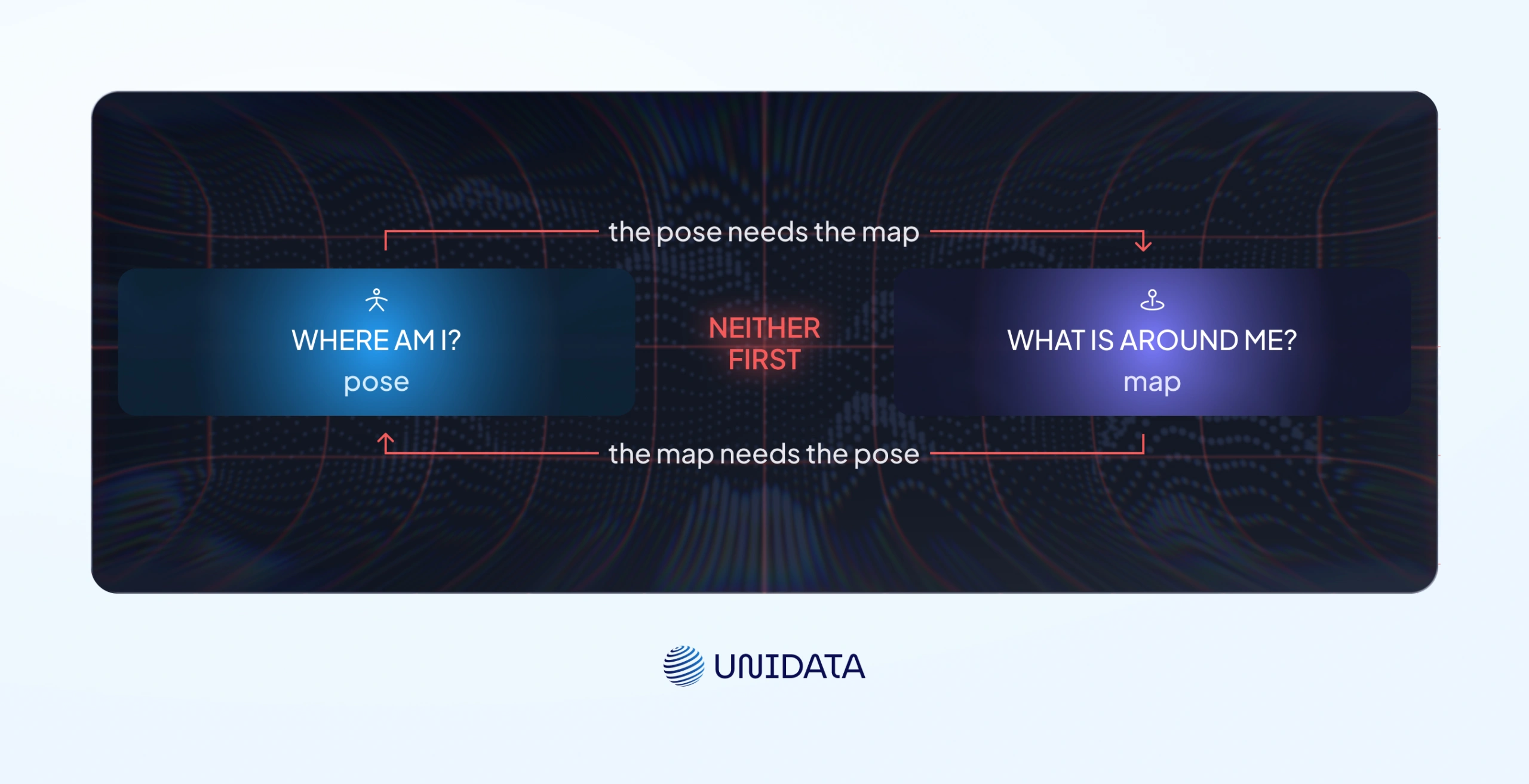
The circularity is the whole reason SLAM is hard. Localization needs a map; mapping needs a location. Two ways out exist, and most real systems use both.

The first is incremental consistency: use the best available position estimate to add the newest scan to the map, then immediately use that improved map to refine the position estimate, and repeat at sensor frame rate (typically 10–20 Hz for spinning LiDAR). Small errors are tolerable because each cycle corrects against the last.

The second is loop closure: when the system recognizes it has returned to a previously mapped place, it can correct the accumulated drift across the entire path traveled since then, not just the last frame. This is the mechanism that turns "approximately right, drifting worse over time" into "globally consistent over an entire building." Loop closure gets its own section below because it is where most of SLAM's practical engineering effort lives.

LiDAR technology: the eyes of the system 

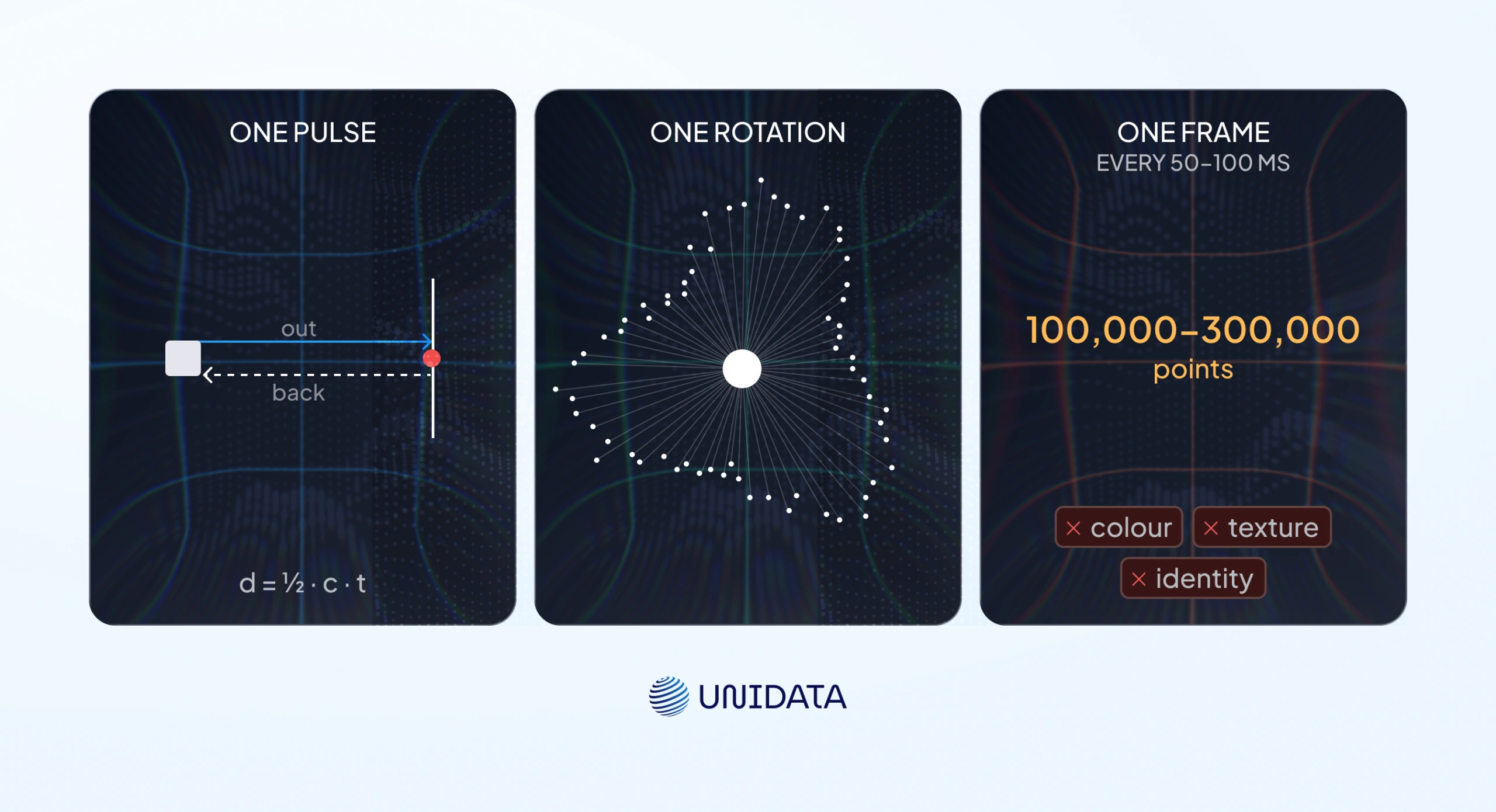
LiDAR — Light Detection and Ranging — measures distance by timing how long a laser pulse takes to leave the sensor, hit a surface, and return. The relationship is direct: distance equals half the speed of light times the round-trip time [2]. Higher-precision time measurement translates directly into finer distance resolution, which is why timing precision is one of the core specs separating LiDAR sensor tiers.

Three time-of-flight approaches are in commercial use: direct time-of-flight (DToF), which times discrete pulses; amplitude-modulated continuous wave (AMCW, sometimes called indirect ToF), which infers distance from phase shift in a continuously modulated signal; and frequency-modulated continuous wave (FMCW), which extracts both distance and velocity from a frequency-swept beam [2]. Spinning mechanical LiDAR units used in most ground robots and autonomous vehicles rotate a laser-detector pair (or an array of them) to sweep a full 360° field of view, firing tens of thousands of pulses per second.

What a SLAM pipeline actually receives from the sensor is a point cloud: a set of 3D coordinates, one per laser return, each marking a surface the beam hit. A single rotation of a typical automotive-grade LiDAR produces on the order of 100,000 to 300,000 points. The SLAM system's job starts the instant that point cloud lands in memory.

2D vs. 3D LiDAR: dimensional differences

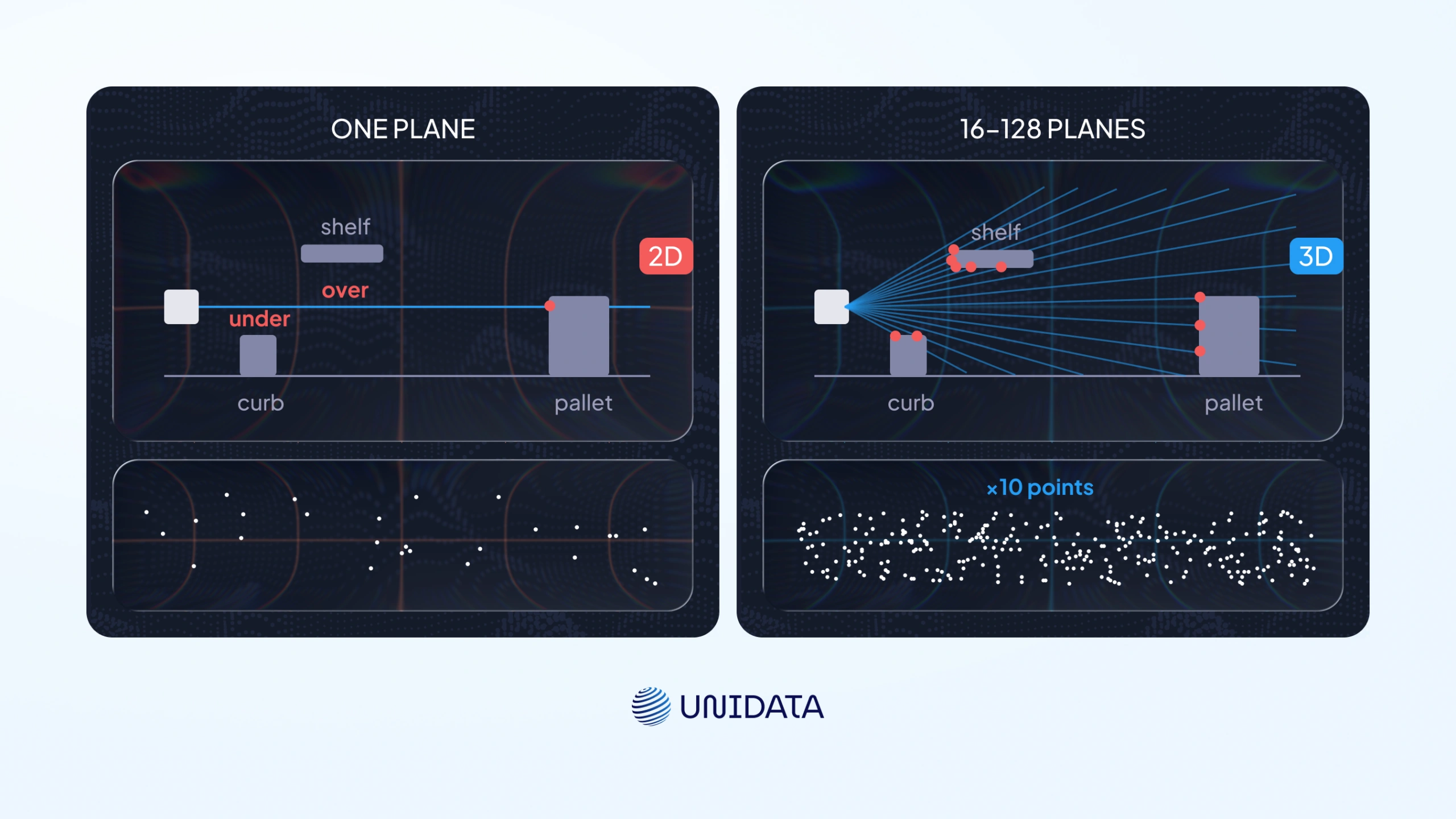
A 2D LiDAR sweeps a single horizontal plane, producing a flat slice of the environment — enough to navigate a flat warehouse floor or a corridor, not enough to detect a low-hanging shelf or a curb. It's cheaper, computationally lighter, and was the default for ground robots for years; Google's Cartographer system, still a reference implementation for many indoor robots, was originally built around 2D LiDAR for exactly this reason [3].

A 3D LiDAR adds vertical channels — anywhere from 16 to 128, depending on the sensor — sweeping multiple planes simultaneously to capture full volumetric geometry: overhangs, stairs, uneven terrain, objects at any height. The trade-off is data volume and compute: a 3D system processes an order of magnitude more points per scan, which is exactly why scan-matching algorithm choice (covered next) matters so much more for 3D pipelines than for 2D ones.

How 3D LiDAR SLAM works

A 3D LiDAR SLAM system is usually described as front-end and back-end, and the split matters because the two halves run on different timescales and solve different problems. The front end runs at sensor frame rate, aligning each new scan to what came before. The back end runs less frequently, correcting the accumulated structure of the whole map when new evidence — typically a loop closure — justifies a global adjustment. 

Key components of the SLAM Pipeline

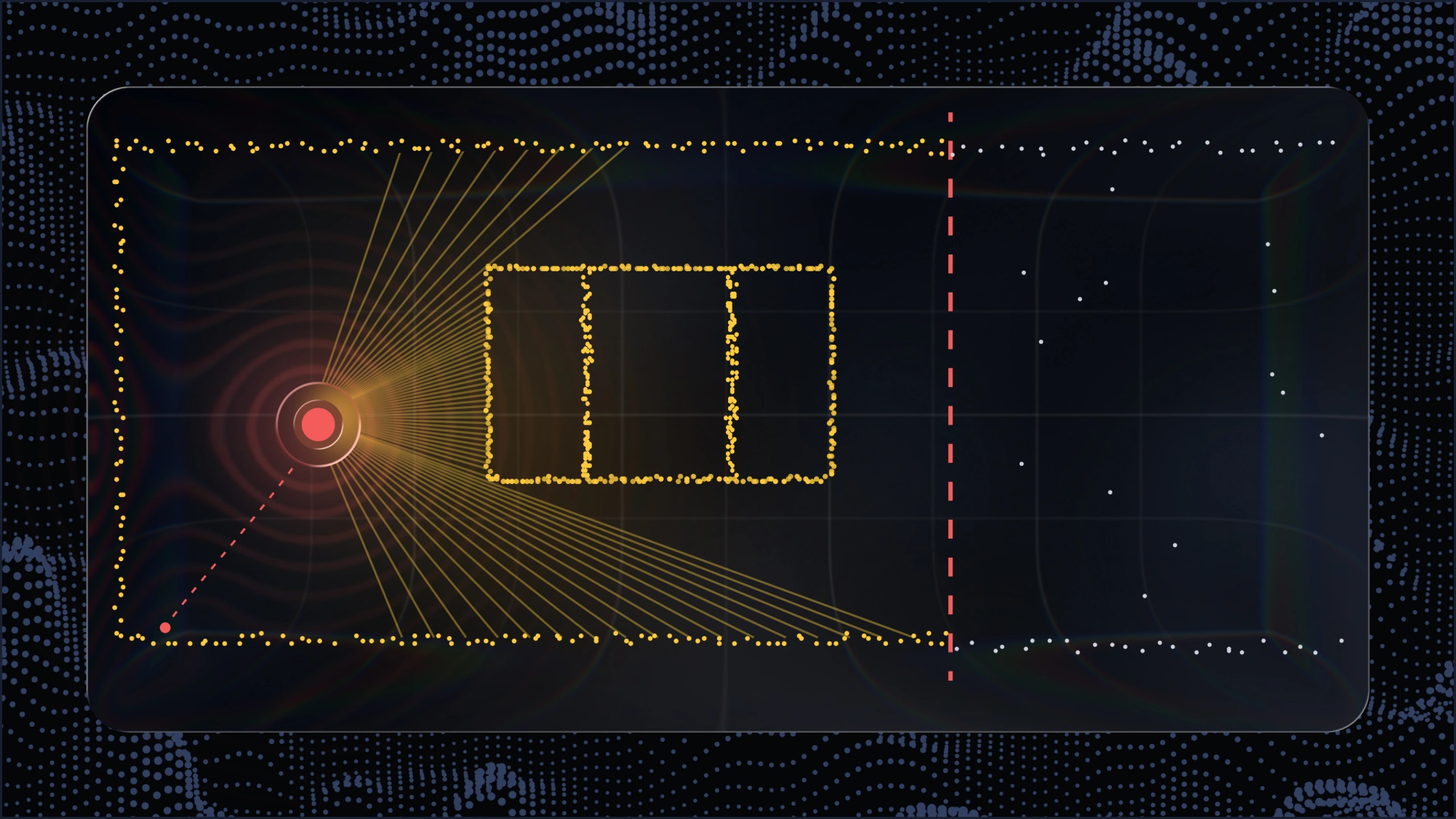
The front end performs three jobs in sequence. First, feature extraction reduces a raw point cloud (hundreds of thousands of points) to a smaller set of distinctive geometric features — edges and planar surfaces are the standard choice, since they're stable across viewpoints and cheap to match. LOAM, one of the most cited LiDAR odometry methods, built its entire real-time performance around this reduction. It extracts edge and planar features and matches only those — rather than every raw point — against the accumulating map [4]. Second, scan matching (detailed below) estimates the sensor's motion between the current scan and the map by finding the geometric transformation that best aligns them. Third, the estimated motion is integrated to update the running position estimate — this is LiDAR odometry, the SLAM equivalent of dead reckoning, and it's what most systems use for moment-to-moment position even before any global correction happens. 

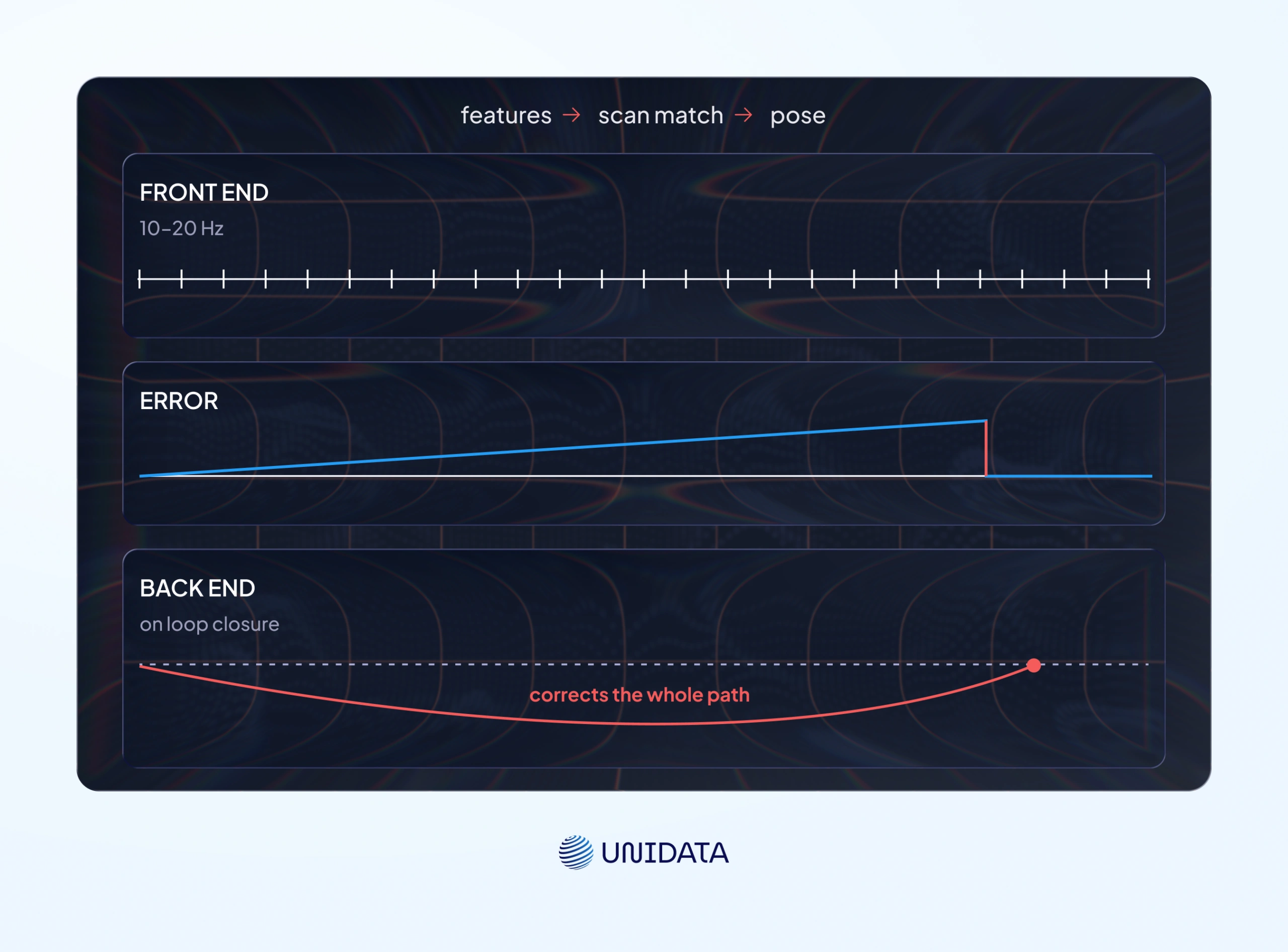
positions at different times and edges are the spatial constraints between them (both from scan matching and from loop closures). When a loop closure adds a new constraint that conflicts with the accumulated drift, the back end runs graph optimization to redistribute that error across the whole path — correcting not just the most recent pose but the entire trajectory since the loop began.

Scan matching algorithms: deep technical dive

Three families of scan-matching algorithms dominate production SLAM, and the choice between them is a real engineering decision, not a default to accept. 

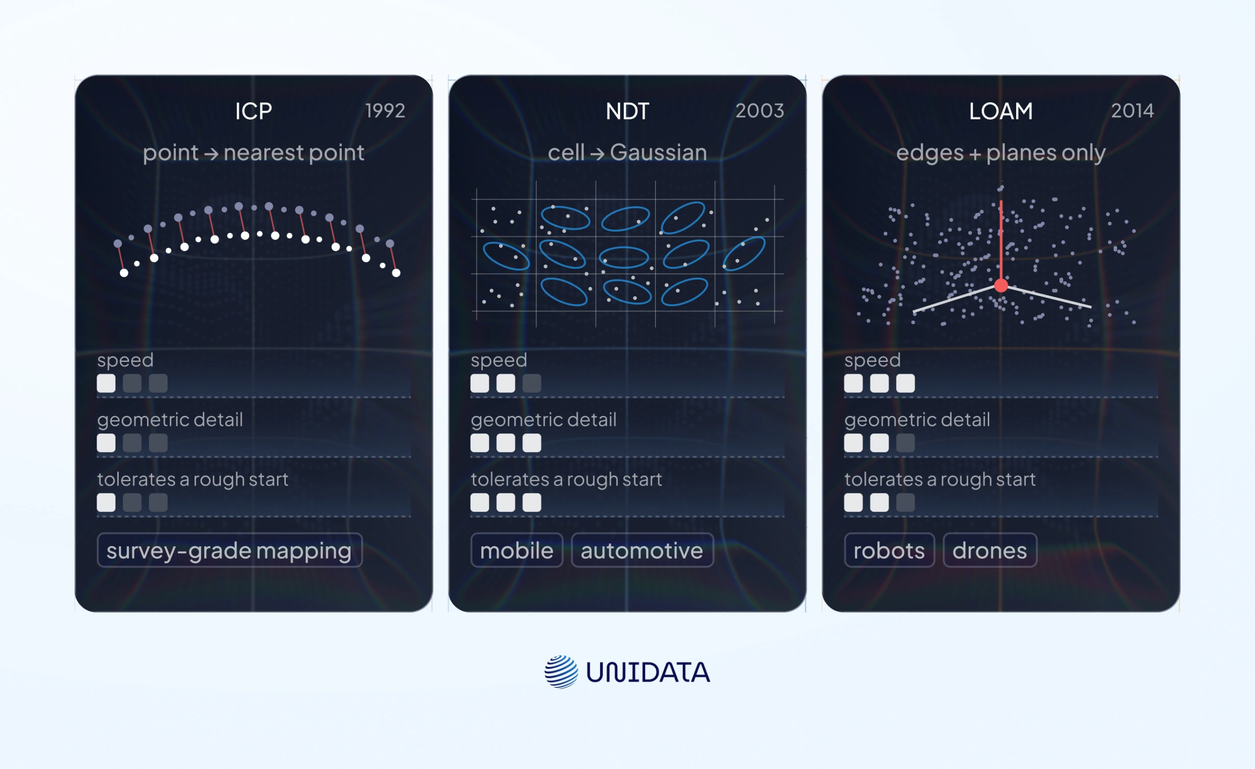
Iterative Closest Point (ICP), introduced by Besl and McKay in 1992, is the oldest and still the conceptual baseline [5]. It alternates between two steps: for each point in a new scan, find its nearest neighbor in the reference point cloud, then compute the rigid transformation that minimizes the total distance between all matched pairs. Repeat until the transformation stops changing. ICP is accurate when the two scans already overlap closely, but it's expensive — nearest-neighbor search over large point clouds is the bottleneck — and it converges to the wrong answer (a local minimum) if the initial alignment guess is too far off, which is common after fast motion or in textureless environments.

Normal Distributions Transform (NDT), published by Biber and Straßer in 2003, takes a different approach: instead of matching individual points, it divides space into a grid of cells, models the distribution of points within each cell as a Gaussian, and optimizes alignment against that smoothed probability model. The original 2003 method worked in 2D; later 3D extensions apply the same cell-based Gaussian model to full volumetric scans [6]. Because it doesn't need point-to-point correspondences, NDT tends to be faster and more tolerant of a rough initial guess than ICP, which is part of why it's a common default in mobile mapping and automotive SLAM pipelines.

Feature-based registration — the LOAM family and its many derivatives — skips dense point matching entirely and matches only extracted edge and planar features [4]. This is the fastest of the three by a wide margin, which is why it dominates in real-time robotics where compute is constrained, at some cost in fine geometric accuracy compared to dense methods.

No single algorithm wins on every axis. Production systems usually pick based on the binding constraint: ICP or NDT when point cloud fidelity matters more than compute budget (survey-grade mapping), feature-based methods when frame rate and onboard compute are the bottleneck (mobile robots, drones).

Point cloud registration and scan matching

Point cloud registration is the general term for finding the transformation that aligns two point clouds — scan matching is registration applied specifically to consecutive (or near-consecutive) LiDAR frames within a SLAM loop. The distinction matters because registration also runs at a longer timescale: when the back end performs loop closure, it's registering the current scan against a map fragment built minutes or hours earlier, not just the previous frame.

A capability that's easy to underrate until it's needed: dense 3D reconstruction from registered point clouds. KinectFusion demonstrated this with a depth camera rather than LiDAR, but the principle transfers directly — continuously registering incoming depth frames against an accumulating volumetric model produces a dense, real-time 3D reconstruction rather than a sparse feature map [7]. The same idea, applied to LiDAR point clouds at larger scale, is what underlies dense mapping for digital twins and as-built surveys, where the deliverable is a usable 3D model of the space, not just a robot's localization estimate.

Loop closure: ensuring map consistency

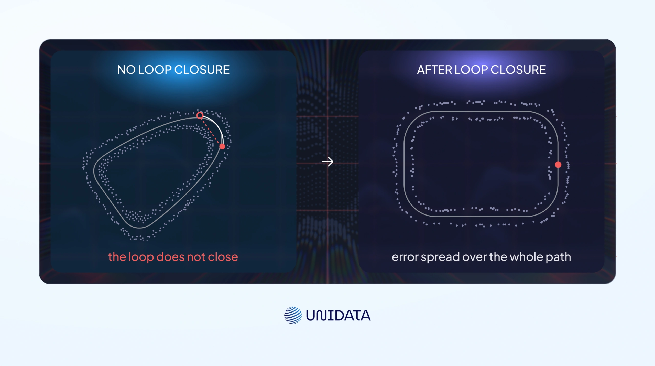
Loop closure detection asks one question continuously: has the sensor returned to a place it has already mapped? Detecting this — typically by matching the current scan's features against a database of previously visited locations — lets the system add a constraint that says "this position now and that position from twenty minutes ago are the same place," even though dead-reckoning drift may have separated their estimated coordinates by meters. 

Cartographer's contribution to this problem, still widely referenced, was making loop closure run efficiently enough for real-time 2D LIDAR SLAM by limiting expensive global optimization to local submaps and only fusing them when a loop closure is detected, rather than re-optimizing the entire map continuously [3]. The same architectural idea — keep local consistency cheap, reserve expensive global correction for confirmed loop closures — carries into most 3D systems.

Without loop closure, a SLAM system's map quality degrades monotonically with distance traveled, because every scan-matching step introduces a small error that the next step inherits. Over a short corridor this is invisible. Over a multi-floor building or a multi-kilometer survey route, uncorrected drift produces a map that visibly fails to close on itself — corridors that should connect don't, and the system has no way to know its own error until loop closure tells it.

Advantages of 3D LiDAR SLAM

3D LiDAR SLAM's core advantage is that it produces metrically accurate geometry directly from the sensor, in conditions that defeat camera-based systems — and it does this without needing external infrastructure like GPS beacons or pre-placed markers. A LiDAR sensor measures real-world distances directly; there's no scale ambiguity to resolve, no dependence on scene texture, and no dependence on ambient light. A LiDAR SLAM system performs comparably in a sunlit loading dock, a dim warehouse aisle, and complete darkness, because illumination has no effect on time-of-flight measurement.

In-depth comparison between LiDAR SLAM and Visual SLAM 

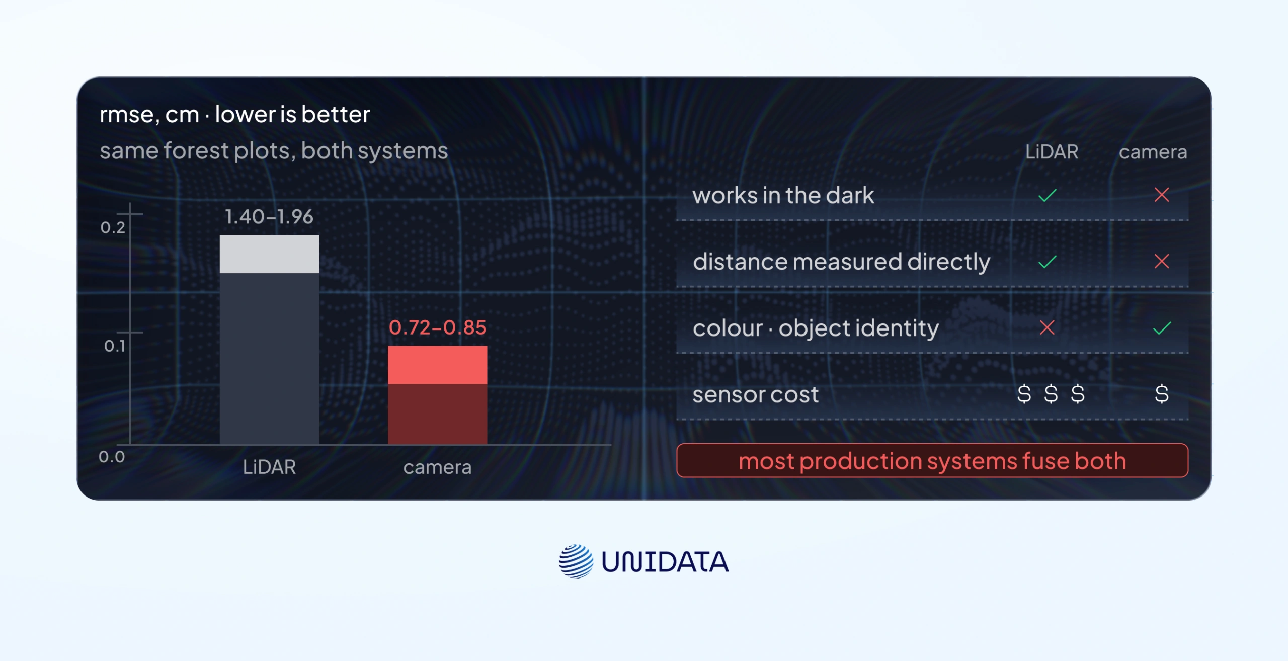
Visual SLAM (vSLAM) uses cameras instead of (or alongside) LiDAR, extracting features from image sequences and triangulating geometry the way human stereo vision does. The trade-offs are close to a mirror image of LiDAR's.

Cameras are dramatically cheaper than LiDAR units and capture rich semantic and textural detail — color, signage, object identity — that LiDAR's geometric point cloud doesn't carry at all. That semantic richness is genuinely valuable for tasks like place recognition and object-aware navigation. But vSLAM's accuracy is lighting-dependent and texture-dependent: it degrades in low light, struggles with feature-poor environments like blank walls or uniform flooring, and (for monocular setups) has to resolve absolute scale indirectly rather than measuring it. A forest-plot survey comparing both approaches found LiDAR SLAM measuring tree diameter at 1.4–1.96 cm RMSE (root-mean-square error, a standard accuracy measure) against survey-grade reference. Visual SLAM matched or slightly outperformed it on that same metric, at 0.72–0.85 cm under the canopy conditions tested [8]. The result is a useful corrective: LiDAR's real edge in that study wasn't raw measurement accuracy on every metric, it was the density and completeness of the point cloud output for downstream modeling — "more accurate" depends on which metric and which environment are being compared.

The practical conclusion most integrators reach is not "pick one" but "fuse both." LiDAR supplies metric accuracy and lighting independence; cameras supply semantic context and lower cost. A growing share of production systems run LiDAR-visual fusion rather than either sensor alone.

Comparison with traditional mapping technologies

Static terrestrial laser scanning (TLS) — a tripod-mounted scanner capturing one stationary, very high-density scan at a time — remains the accuracy ceiling for as-built survey work, with millimeter-level precision under controlled conditions. Mobile SLAM-based mapping systems move continuously through a space instead, trading some of that accuracy for a substantial speed advantage. 

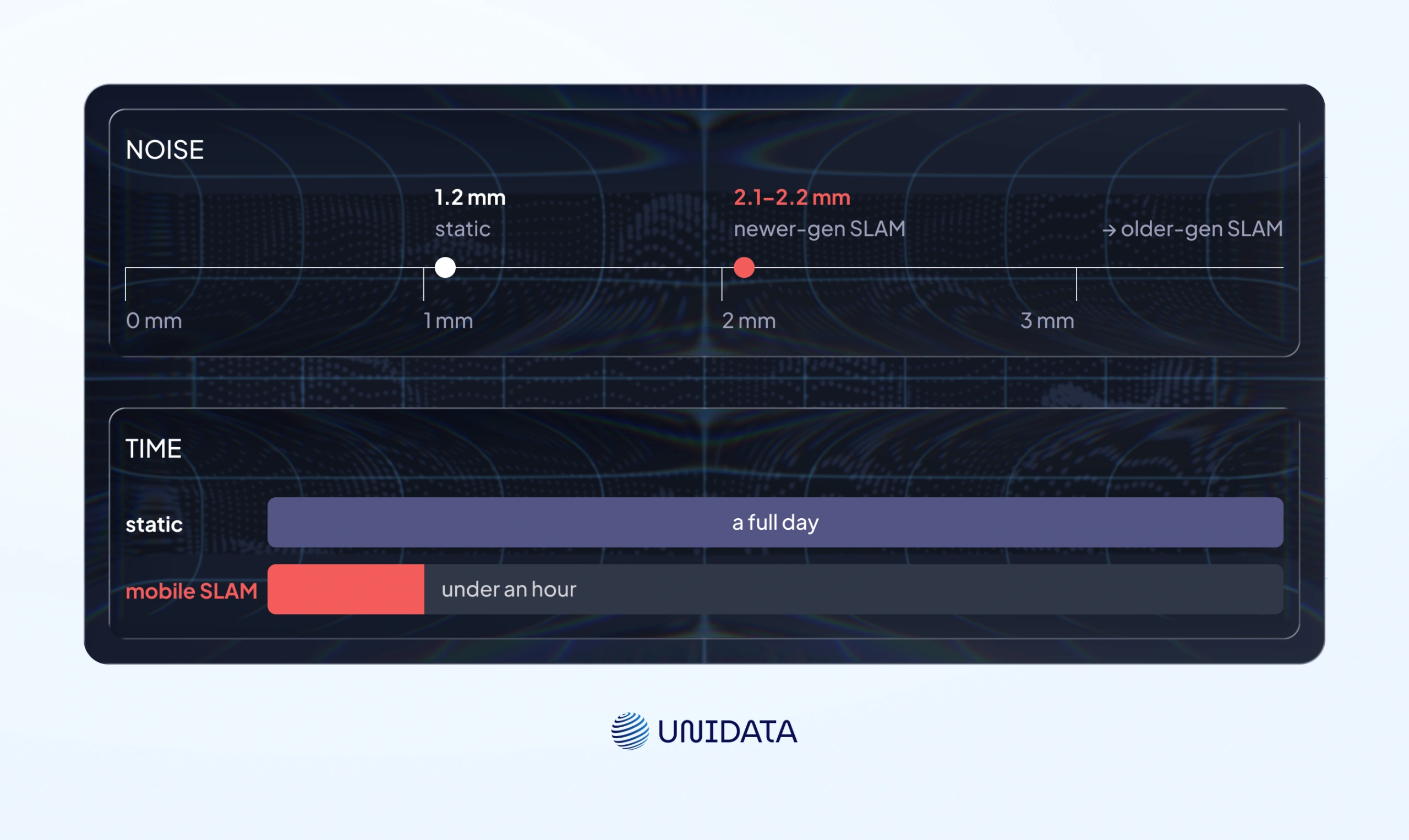
How much accuracy gets traded away turns out to depend heavily on scanner generation: a controlled indoor comparison found an older-generation SLAM scanner trailing static reference accuracy by a wide margin, while two newer-generation SLAM units closed most of that gap, with post-processing noise levels around 2.1–2.2 mm against a 1.2 mm static reference — close enough that generational hardware improvement matters more to the accuracy question than the static-versus-mobile distinction itself [9].

For most commercial use cases — facility surveys, construction progress tracking, retrofit planning — the speed advantage outweighs the accuracy gap: a space that takes a TLS crew a full day to scan station-by-station can often be walked through with a mobile SLAM rig in under an hour. TLS still wins outright when the deliverable requires millimeter-level legal or engineering tolerance, such as structural deformation monitoring.

Common сhallenges and solutions

Most of the problems that show up in production 3D LiDAR SLAM deployments aren't algorithmic in the textbook sense — they're environmental conditions the core scan-matching math doesn't handle gracefully on its own. 

Feature-poor environments — long straight corridors, open warehouse floors, repetitive shelving — give scan matching too little distinctive geometry to anchor against, which is exactly the condition that produces local-minimum failures in ICP and degraded confidence in NDT. The usual mitigations are sensor fusion (adding an IMU — inertial measurement unit, a chip that tracks acceleration and rotation — or wheel odometry to constrain motion when LiDAR alone is ambiguous) and deliberately engineering some asymmetry into the environment where possible. 

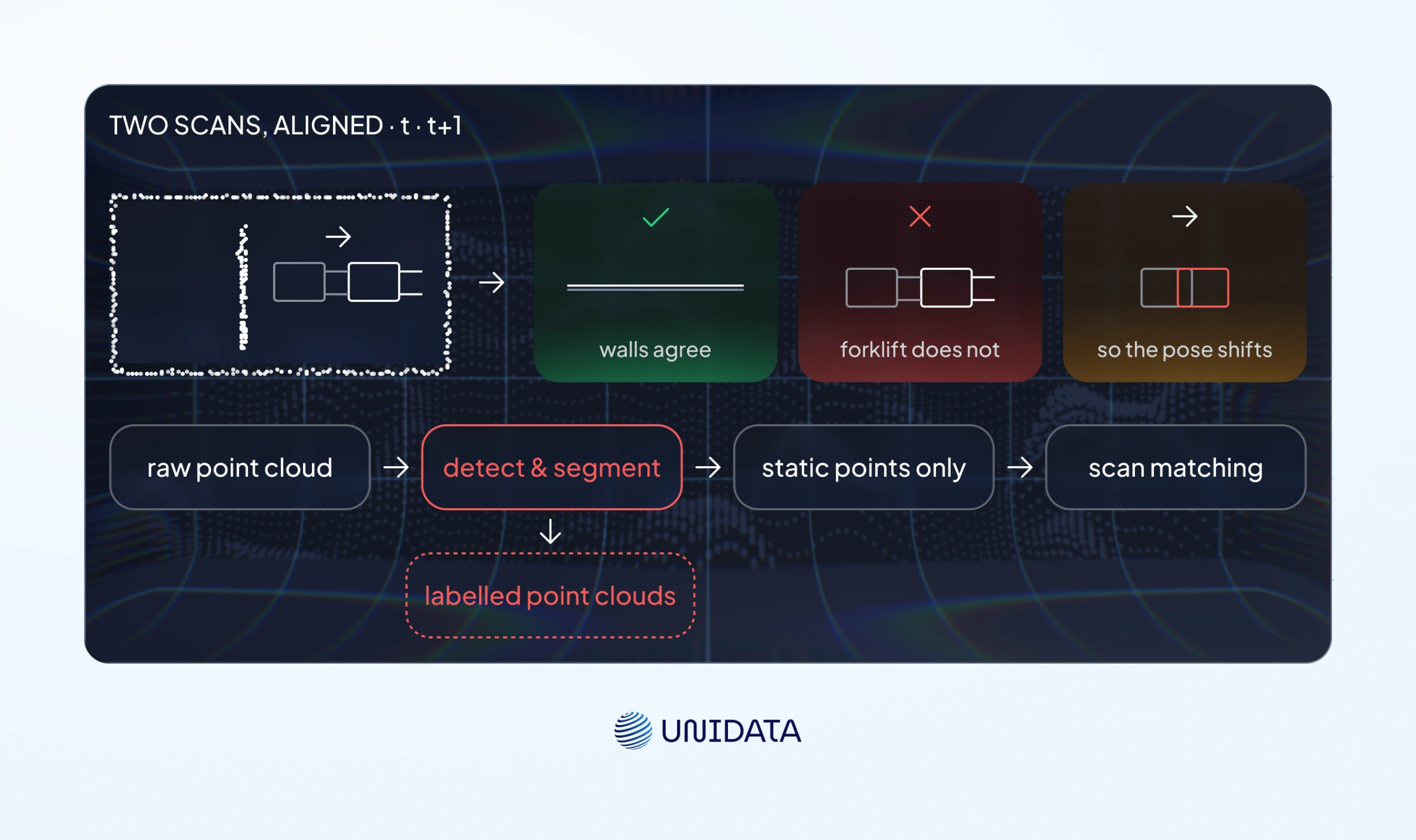
Dynamic objects are the more persistent problem. A scan-matching algorithm assumes the environment is static between scans; a person, forklift, or another robot moving through the scene violates that assumption and corrupts the match. The fix requires detecting and either filtering out or separately tracking moving objects before they reach the scan-matching stage — which means the pipeline needs an object detection or semantic segmentation model running on the point cloud, not just geometric registration [10]. That detection model is only as good as the labeled point cloud data it was trained on: distinguishing "static shelf" from "person mid-stride" from "pallet being moved" in raw LiDAR returns is a model problem, and the model problem is a data problem first. This is the layer where teams we work with most often hit a wall — not because the SLAM math is wrong, but because nobody annotated enough LiDAR point cloud examples of the specific moving objects their environment actually contains.

Computational and memory constraints show up as map size grows — a multi-floor facility's accumulated point cloud can run into the hundreds of millions of points, more than most onboard compute can hold or process at frame rate. Voxel-grid downsampling (thinning point density by snapping points to a fixed 3D grid cell), keyframe-based map management (storing only a representative subset of historical scans rather than every frame), and offloading global optimization to less time-critical compute are the standard answers.

Applications across industries

Autonomous vehicles and robotics

Self-driving vehicles and warehouse AGVs (automated guided vehicles) were among the first commercial drivers of 3D LiDAR SLAM, for a straightforward reason: both need to localize precisely without depending on GPS, which is unreliable in parking structures, dense urban canyons, and most indoor facilities. A delivery robot navigating a warehouse aisle and a passenger vehicle navigating a city block are running variants of the same SLAM pipeline, tuned for very different speeds and obstacle types.

Underground and confined environments push the same technology into harder territory. Mining and tunneling robotics rely on LiDAR SLAM specifically because no other localization method works underground at all — no GPS, often no reliable lighting, and frequently no prior map of a space still being excavated. Research into mining-specific SLAM has focused on registration methods that hold up against the repetitive, feature-poor geometry of tunnel walls, an even harder version of the feature-poor-environment problem described above [11].

Mapping, surveying, and digital Twins

Outside of moving vehicles, 3D LiDAR SLAM has become a practical tool for capturing existing spaces as accurate 3D models — digital twins used for facility management, renovation planning, and increasingly, training data for robots that will operate in those same spaces.

That last use case is where mapping and robotics start to overlap directly. A robot learning to navigate an apartment, a warehouse aisle, or a retail floor benefits from training against the real geometry of the space it will actually operate in, not a generic synthetic approximation. Unidata's team has worked on exactly this kind of capture: scanning real apartment interiors to produce point cloud data that gives robot navigation training real spatial ground truth instead of a synthetic stand-in — the kind of underlying scan data that mobile SLAM mapping makes practical to collect at the speed projects actually need.

3D LiDAR SLAM for drone operations

Drones add a constraint ground robots don't have: GPS-denied operation combined with six degrees of freedom of motion and tight payload limits on sensor weight and compute. UAV LiDAR SLAM research has converged on lightweight, often solid-state LiDAR units paired with tightly integrated IMU fusion, since a drone can't rely on wheel odometry the way a ground vehicle can, and any scan-matching drift compounds faster in free 3D flight than in planar ground motion [12]. Tunnel and confined-space inspection drones are a particularly demanding case: fully GPS-denied, often with repetitive feature-poor walls, and requiring real-time obstacle avoidance on top of mapping.

Business ROI and competitive advantages

The business case for 3D LiDAR SLAM over alternatives usually comes down to deployment speed and operating cost rather than raw accuracy. A facility that would need physical infrastructure — floor markers, beacons, reflective targets — for older localization methods can deploy a LiDAR SLAM-equipped robot with no environment modification at all, which matters directly for time-to-deployment in leased or shared facilities. The same property that makes LiDAR SLAM technically attractive (no external infrastructure dependency) is what makes it commercially attractive: lower setup cost per site and faster redeployment when a facility layout changes.

Future trends in 3D LiDAR SLAM

Technical maturity and evolution timeline

The clearest near-term trend is market growth on the sensor side, even though cost remains a real barrier rather than a solved problem. Solid-state LiDAR — which replaces mechanical spinning assemblies with fixed-beam-steering electronics — has been moving from automotive prototype hardware toward mainstream deployment. Industry sizing puts the solid-state LiDAR market at roughly $2.65 billion in 2026, growing toward $11 billion by 2034, with autonomous-vehicle applications as the largest demand driver. Per-unit average selling prices still run $1,000 to $10,000 depending on performance and resolution requirements — high enough that analysts cite cost as the main restraint on wider automotive adoption today [13].

Cheaper, more reliable sensors would widen which industries can justify a LiDAR SLAM deployment at all; that calculation changes substantially once sensor cost stops dominating the total system price, which is the direction the market is heading even though it hasn't gotten there yet.

Beyond SLAM: semantic understanding and intelligence

The maturity curve for SLAM is bending away from "more precise geometry" and toward "more meaningful geometry." A geometrically perfect map that can't distinguish a door from a wall, or a person from a stationary obstacle, has a ceiling on how autonomous the system built on top of it can become. Semantic SLAM addresses exactly this: fusing object recognition and scene understanding directly into the mapping process, so the output is a map labeled with object classes and semantic regions, not just occupied and unoccupied space [14].

This is also where the gap between "the SLAM algorithm works" and "the deployed system works" tends to live. Semantic SLAM's object recognition layer is a trained model, and a trained model is only as capable as its training data — specifically, point cloud and video data with the object classes, instance boundaries, and edge cases the deployment environment actually contains. Teams building toward semantic SLAM are, in practice, also building an annotated-data pipeline: enough labeled 3D point cloud examples of the specific objects, materials, and clutter their robots will encounter to train a recognition model that doesn't fail on the long tail — the layer underneath semantic SLAM that gets less attention than the algorithm, even though it determines how the algorithm actually performs once deployed.

Implementing 3D LiDAR SLAM: practical considerations

Selecting the right hardware and software

The hardware decision starts with channel count and range, both of which trade directly against cost and compute load. A 16-channel LiDAR is enough for basic indoor ground robotics; dense outdoor mapping or automotive applications typically need 32 to 128 channels and proportionally more onboard compute to process the resulting point cloud at frame rate. Solid-state units are increasingly competitive on cost for shorter-range applications, while mechanical spinning LiDAR still leads on long-range outdoor performance.

On the software side, the realistic choice for most teams isn't "write a SLAM system from scratch" — it's choosing among mature open-source frameworks (Cartographer, LOAM and its derivatives, various ROS-integrated SLAM packages) and adapting parameters and front-end algorithm choice to the deployment environment's specific feature density and dynamics. Building from scratch is rarely the efficient path unless the use case sits well outside what existing frameworks support.

Practical implementation workflow

A realistic rollout sequence runs roughly as follows:

1. Characterize the deployment environment first — feature density, expected dynamic object types, lighting variability, GPS availability — before selecting a scan-matching algorithm, since that characterization is what the algorithm choice in the Scan Matching section above should actually be based on.
2. Prototype with an existing open-source SLAM stack rather than custom code.
3. Test loop closure performance specifically on the actual planned routes, not just open-floor test runs. Loop closure failure modes are route-dependent, and an open-floor run won't surface them.
4. Budget separately, and early, for the object detection and semantic layer if the deployment includes dynamic objects or needs object-aware behavior. That layer needs its own labeled training data, and data collection has its own lead time — distinct from getting the core SLAM pipeline running.

Technical glossary of 3D LiDAR SLAM terms

Point cloud — a set of 3D coordinates representing surfaces a LiDAR sensor's laser pulses have reflected off.

Scan matching — the process of finding the geometric transformation that best aligns two point clouds (typically consecutive sensor frames).

Loop closure — recognizing that the sensor has returned to a previously mapped location, enabling correction of accumulated drift across the path traveled since.

Pose graph — a graph representation where nodes are estimated sensor positions over time and edges are the spatial constraints between them, optimized to produce a globally consistent map.

LiDAR odometry — incremental motion estimation from consecutive LiDAR scans, analogous to wheel-based dead reckoning but derived from laser range data.

ICP (Iterative Closest Point) — a scan-matching algorithm that iteratively finds nearest-neighbor point correspondences and minimizes the distance between them.

NDT (Normal Distributions Transform) — a scan-matching algorithm that models point cloud cells as probability distributions rather than matching individual points.

Semantic SLAM — SLAM augmented with object recognition, producing maps labeled with object classes and regions rather than only geometric occupancy.

Drift — the accumulated position error in a SLAM system over time or distance, caused by small errors compounding across successive scan matches.

Conclusion: the impact of 3D LiDAR SLAM

3D LiDAR SLAM turned "build a map while finding your way through it" from a research problem into deployable infrastructure for any system that has to operate without GPS and without a pre-built floor plan. The core pipeline — extract features, match scans, track drift, close loops — is mature enough now that the harder open questions have moved up a level. The question is no longer "can the system localize itself," but "does the map it builds understand what it's looking at." That shift toward semantic understanding is also a shift toward data: the algorithm that recognizes a moving forklift or an open doorway is only as reliable as the labeled point cloud examples it learned from.

If your SLAM pipeline needs annotated LiDAR point cloud data to train the object-recognition layer that geometry alone can't provide — start here. 

Checked by Expert

Kirill Meshyk

Head of AI Data Collection

LinkedIn

• Data Collection
• AI Data Collection
• Crowdsourcing
• Biometric Data
• Synthetic Data