
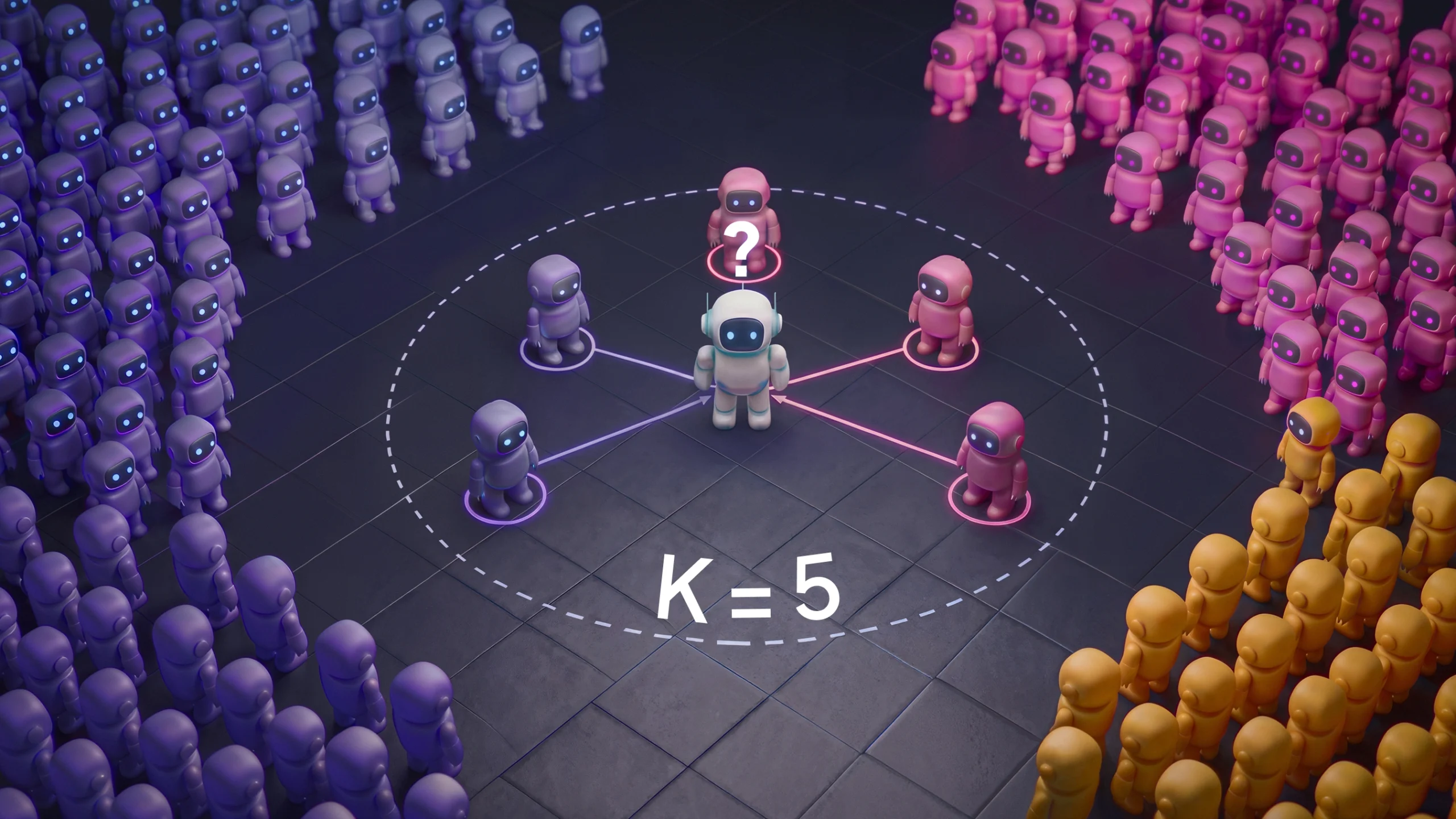
The KNN algorithm — short for K-nearest neighbors — is one of the most intuitive and widely taught algorithms in machine learning. Its core idea is simple: if you want to know what class an unknown data point belongs to, look at the closest known points and let them vote.
First described by Fix and Hodges in 1951 and formally analyzed by Cover and Hart in a landmark 1967 IEEE paper, the algorithm has outlasted dozens of competitors. The reason is straightforward: algorithms that are easy to understand, debug, and explain to stakeholders tend to stick around.
Despite its simplicity, the KNN algorithm is used in production systems ranging from recommendation systems to decision-support applications. It handles both classification (predicting a category) and regression (predicting a number), requires no explicit model-training phase beyond storing the data, and makes no explicit assumptions about the functional form or probability distribution of the data.
This guide covers everything from core concepts and mathematics through step-by-step implementation to real-world applications and optimization techniques. Code examples use Python and scikit-learn throughout.
What KNN Is — and How It Thinks
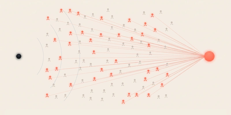
Think about how you decide which neighborhood in a city to live in. You look at who already lives nearby. If three of your four closest potential neighbors are teachers, you probably assume the area is teacher-friendly. The KNN algorithm works the same way; it classifies or predicts based on the majority characteristics of the closest data points in a training dataset.
Formally, KNN is a supervised learning algorithm. That means it learns from labeled training examples. Given a new, unlabeled data point, KNN finds the K training examples most similar to it — the "nearest neighbors" — and uses their labels to make a prediction.
The query point (★) is assigned to Class A because 3 of its 5 nearest neighbours (orange rings) belong to that class. The dashed circle shows the K=5 search radius. This is the core mechanism of the KNN algorithm.
The algorithm belongs to a family called instance-based learning or lazy learning. Unlike most machine learning algorithms, KNN does not build an internal model during training. It simply stores the training data and defers all computation to prediction time. This has real consequences for speed and memory, which we'll cover in detail later.
The Majority Voting Mechanism
For classification, KNN uses majority voting. After identifying the K nearest neighbors, the algorithm counts the class labels and returns the most common one. If K=5 and three neighbors belong to class A while two belong to class B, the prediction is class A.
For regression, KNN computes the arithmetic mean of the K neighbours' output values. Weighted KNN gives closer neighbours more influence by assigning each a weight proportional to 1/distance. Note: scikit-learn's weights='distance' option uses 1/d weighting. A separate 1/d² scheme (where a neighbour 0.1 units away has 100 times more influence than one 1.0 units away) can be implemented with a custom weight function. Either approach usually improves accuracy on datasets with complex decision boundaries.
The Mathematics Behind KNN
Distance is everything in KNN. The algorithm can't determine which points are "nearest" without a way to measure closeness. That measurement comes from distance metrics — mathematical functions that quantify how far apart two data points are in feature space.
The three most important distance metrics in KNN are Euclidean, Manhattan, and Minkowski.
Distance Metrics Used in the KNN Algorithm
Each metric measures "closeness" differently — the choice impacts which points are considered neighbours
Always scale your features before computing distances. A feature measured in thousands will dominate any distance calculation over a feature measured in decimals, regardless of how meaningful each feature actually is. Apply StandardScaler or MinMaxScaler before fitting any KNN model.
| Euclidean Distance | Manhattan Distance | Minkowski Distance |
|---|---|---|
| $$d_{\text{Euclidean}}(\mathbf{x}, \mathbf{y})= \sqrt{\sum_{i=1}^{n} (x_i - y_i)^2}$$ The straight-line distance between two points. Think of it as measuring with a ruler in geometric space. This is the default for most KNN implementations and works well when features are continuous and scaled. | $$d_{\text{Manhattan}}(\mathbf{x}, \mathbf{y})= \sum_{i=1}^{n} |x_i - y_i|$$ The "city block" distance — sum of absolute differences along each dimension. More robust to outliers than Euclidean distance. Often preferred for high-dimensional data or when features are not correlated. | $$ d_{\text{Minkowski}}(x,y)=\left(\sum_{i=1}^{n}|x_i-y_i|^p\right)^{1/p},\quad p\ge 1 $$ A generalization of both. When p=1, it equals Manhattan distance; when p=2, it equals Euclidean. The parameter p gives you flexibility to tune distance sensitivity. |
Lazy Learning and KNN Algorithm
Most machine learning algorithms — neural networks, decision trees, random forests, SVMs — are eager learners. They process training data upfront, extract patterns, and compress them into a compact model. At prediction time, the model is small and fast.
KNN takes the opposite approach. Training consists of a single operation: store all the data. The entire workload is deferred to prediction time. When a query arrives, the full training set must be searched.
Lazy Learning (KNN) vs. Eager Learning (Decision Tree)
| Property | KNN (Lazy) | Decision Tree (Eager) |
|---|---|---|
| Training time | Near zero — stores data only | Moderate to high — builds tree |
| Prediction time | Slow — searches all training data | Fast — traverses tree nodes |
| Memory usage | High — stores all examples | Low — compact model |
| Adapts to new data | Immediately, no retraining | Requires full or partial retraining |
| Interpretability | High — show the K neighbors | High — show the decision path |
| Distribution assumptions | No — non-parametric | Implicitly assumes axis-aligned cuts |
The practical implication of lazy learning: KNN adapts to new data immediately. Append new training examples and the next prediction automatically considers them — no retraining cycle. The cost is prediction speed. Each query requires O(n · d) operations, where n is training set size and d is the number of features.
How KNN Works: Step by Step

To understand how KNN actually works, it helps to walk through an example step by step.
Imagine you’ve logged 1,000 past training runs. Some of those models ended up overfitting, while others generalized well. Each run is described using two simple features: the size of the training dataset and the model’s complexity, measured by its parameter count.
Now, a new experiment comes in. The dataset contains 8,200 examples, and the model has 4.3 million parameters.
The question is straightforward: based on what has happened before, is this model more likely to overfit or generalize?
Step 1 — Load and Prepare the Dataset
To compare apples to apples, all data must be numeric and complete. Right now, they aren’t. Dataset size might go up to hundreds of thousands, while complexity is measured in millions of parameters. Without adjustment, one feature would dominate the distance calculation.
To fix that, apply Z-score standardization so each feature contributes equally.
Standardization Formula
Where:
- μ is the training-set mean
- σ is the standard deviation of the training set
Step 2 — Choose the Value of K
Next, decide how many neighbors should influence the prediction. A common starting point is the square-root heuristic:
The Square-Root Heuristic
Where:
- where n is the number of training examples
For 1,000 training runs, that gives K ≈ 31. In binary classification, it’s better to keep K odd to avoid ties during voting.
This rule is not theoretically optimal and should be treated only as an initial estimate. The final value of K should be selected through cross-validation.
Step 3 — Calculate Distances
Now the core operation: compare the new experiment to every historical run. This is done by computing the Euclidean distance in the standardized feature space:
Euclidean Distance Formula
Where:
- where d is the number of features (2 here: dataset size and complexity score)
- $$x_{ij}$$ is feature j of training point i
- $$x_{nj}$$ is feature j of the query.
Running this calculation across all records produces 1,000 distance values—one per training example.
Step 4 — Sort and Identify K Nearest Neighbors
With all distances computed, sort them from smallest to largest. The algorithm then isolates the K-neighborhood, which consists of the 31 historical runs that are most similar to the new experiment.
Neighborhood Set Definition
Essentially, the 31 training runs with the shortest distances to the new point are selected. These specific neighbors will provide the data for the final prediction.
Step 5 — Apply Majority Vote or Averaging
Once the neighborhood is identified, the algorithm aggregates the labels of the K nearest neighbors to reach a decision. For classification tasks like predicting Overfit vs Generalizes, this is done via majority voting. The model selects the class that appears most frequently among the neighbors.
Classification Decision (Argmax)
- $$1[y_i = c]$$ : An indicator function that equals 1 if the neighbor's class matches c, and 0 otherwise.
- $$\text{argmax}_c$$ : Selects the class c with the highest total count.
If the task is regression (for example, predicting a continuous metric like validation loss gap), the algorithm switches from voting to averaging:
If the task is regression (for example, predicting a continuous metric like validation loss gap), the algorithm switches from voting to averaging:
This computes the simple arithmetic mean of the neighbors’ values.
For weighted KNN, closer neighbors are given more influence. A common choice is inverse-distance weighting:
Weight definition:
These weights are then normalized so that they sum to 1, and the prediction becomes a weighted sum instead of a simple average.
Step 6 — Return the Prediction
The final predicted label or value is returned along with any associated confidence estimates (such as the percentage of neighbors that agreed on the class).
Unlike other algorithms, there is no "model" to save or parameters to train. The system is a lazy learner, meaning it performs all necessary logic—scaling, distance calculation, and sorting—at the exact moment a new query is received, using the raw training data as its internal map.
KNN in Machine Learning Workflows
In practice, KNN is rarely used in isolation. It fits into a broader machine learning pipeline — a sequence of steps from raw data to deployed predictions. Understanding where KNN sits in that pipeline helps you set it up for success.
A typical pipeline with KNN looks like this: raw data → preprocessing (cleaning, encoding, scaling) → feature engineering → KNN model → cross-validation → hyperparameter tuning → deployment. Two of these steps deserve special attention.
Feature scaling is usually essential for KNN unless all features are already measured on comparable scales.. Because the algorithm relies entirely on distance, any feature with a larger numeric range will dominate predictions. Before fitting a KNN model, always apply standardization (z-score) or min-max normalization to your features.
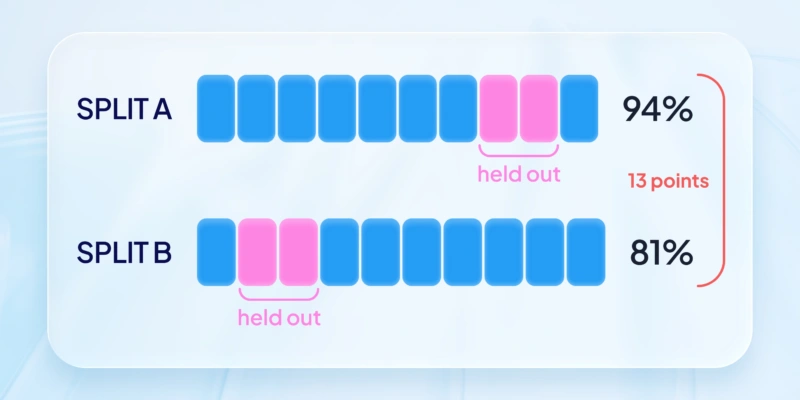
Cross-validation is the standard way to evaluate KNN performance and tune the K hyperparameter. K-fold cross-validation splits your data into K folds, trains on K−1 of them, and tests on the remaining fold — repeated K times. This gives a robust estimate of model performance and helps you find the optimal K value without overfitting to a single train/test split.
KNN is also commonly used as a baseline model. Before deploying a complex neural network or gradient boosting system, a quick KNN fit tells you what a simple, interpretable algorithm can achieve. If your sophisticated model can't beat KNN, you may have a data quality problem rather than an algorithm problem.
Implementation Considerations
Computational Complexity and Scalability
When you move from tutorial notebooks to production environments, the brute-force approach to KNN — computing distances to every training point for every query — quickly becomes a bottleneck. On a dataset with 100,000 training samples and 100 features, each prediction requires 100,000 distance calculations. At scale, this is slow.
Several data structures and algorithms address this. The right choice depends on your dataset size and dimensionality:
KNN Implementation Approaches
| Approach | Search Speed | High Dimensions? | Best For |
|---|---|---|---|
| Brute Force | O(n*d) per query | Any dimension | Small datasets (<10K), prototyping |
| KD-Tree | O(log n) low dims | Degrades >~20 features | Medium datasets, <20 features |
| Ball Tree | Good in high dims | Handles moderate dims | High-dimensional, complex feature spaces |
| LSH (Approx.) | Very fast | Scales to 1000+ features | Very large datasets, approximate OK |
In scikit-learn, the algorithm parameter accepts 'brute', 'kd_tree', 'ball_tree', or 'auto'. (which selects the best option automatically). For most cases, 'auto' is a safe starting point.
Choosing the Optimal K Value
Selecting K is the most consequential hyperparameter decision in KNN because it directly controls the bias-variance trade-off — the fundamental tension between models that memorize training data and models that generalize.
A small K (for example, K=1) makes the model memorize every training point. The decision boundary follows the training data exactly, producing near-perfect training accuracy but poor test accuracy — the classic signature of overfitting. At K=1, every prediction is determined by a single neighbor, making the model extremely sensitive to noise, mislabeled examples, and outliers.
A large K (for example, K=50 in a dataset of 200 points) forces the model to consider so many neighbors that local patterns are averaged away. The decision boundary becomes a smooth, coarse approximation of the true structure — underfitting.
The optimal K lies between these extremes. A practical starting heuristic is K≈n, but the best value depends on the dataset. The real answer comes from systematic search: evaluate a range of odd K values using 10-fold cross-validation with GridSearchCV and select the value that minimizes validation error.
To find the mathematical "sweet spot," the algorithm uses two guiding formulas:
Formula — Bias-Variance Decomposition:
The total expected error is decomposed into three parts:
$$$E[ (y - \hat{f}(x))^2 ] = \text{Bias}[\hat{f}(x)]^2 + \text{Var}[\hat{f}(x)] + \sigma^2_\epsilon$$$
- Bias increases as $$K \uparrow$$ (The model becomes too simple)
- Variance increases as $$K \downarrow$$ (The model becomes too sensitive)
- $$\sigma^2_\epsilon$$ is the irreducible error (inherent noise)
Formula — Optimal K Selection:
While $$K = \sqrt{n}$$ is a common starting heuristic, the mathematically optimal $$K^$$ is found by minimizing the cross-validation error across a range of values (typically odd numbers from $$1$$ to $$\sqrt{n})$$
By testing these values using 10-fold cross-validation, the algorithm identifies the K that balances stability with accuracy, ensuring the model generalizes well to the new experiment's 8,200 examples.
Feature Scaling and Normalization
Feature scaling is mandatory for KNN. No other preprocessing step has a greater impact on performance, and none is more commonly skipped by beginners. The reason: KNN's entire decision-making mechanism is based on distances, and distances depend directly on the numeric scale of each feature.
Consider a dataset with two features: annual income (range: $20,000–$150,000) and age (range: 18–80). Without scaling, a $1,000 difference in income contributes far more to the Euclidean distance than a 10-year age difference. The algorithm will effectively ignore age, even if it is genuinely important for the prediction.
Two scaling methods cover most real-world scenarios:Standardization (Z-score normalization) transforms each feature to mean zero and standard deviation one. Use it for normally distributed data or when you cannot specify a meaningful bounded range in advance — scikit-learn's StandardScaler.
Where:
- μ is the feature mean
- σ is the feature standard deviation
Min-Max Normalization rescales features to [0, 1]. Use it when the feature has a known bounded range, and you need values to remain interpretable as proportions — scikit-learn's MinMaxScaler.
Where:
- The original value of the feature.
- $$x_{\text{min}}$$ : The minimum value of that feature in the dataset.
- $$x_{\text{max}}$$ : The maximum value of that feature in the dataset.
Note that min-max scaling is more sensitive to outliers, since a single extreme value can compress all other values toward zero.
Real-World Applications

Recommendation Systems
Historically, recommendation systems at companies such as Netflix and Amazon have used nearest-neighbor collaborative filtering techniques, often as components of larger hybrid recommendation systems. Modern production systems typically combine collaborative filtering with matrix factorization, deep learning, and other recommendation approaches.
The idea is simple. In user-based filtering, each user is represented as a vector of ratings or interactions. KNN identifies the most similar users and recommends items they liked, but you haven’t interacted with yet.
In item-based filtering, the perspective shifts. Items are represented as vectors in user space, and the algorithm recommends items similar to those you already liked. In practice, this approach tends to be more stable, since item catalogs evolve more slowly than user behavior.
The main limitation is sparsity. Most users interact with only a tiny fraction of available items, leaving the user–item matrix largely empty. As a result, similarity estimates can become unreliable. Techniques like cosine similarity and matrix factorization are commonly used to mitigate this.
Medical Diagnosis
KNN is often used as an interpretable baseline model in clinical prediction tasks because it makes minimal assumptions about the underlying data distribution and provides example-based explanations for its predictions.
Instead of returning an abstract probability, the model surfaces the K most similar historical patients along with their outcomes. This aligns closely with how clinicians already think: reasoning by analogy and prior cases.
That transparency can be critical in high-stakes environments where decisions need to be explainable, not just accurate.
Anomaly Detection and Fraud Prevention
KNN also lends itself naturally to anomaly detection. A data point that has no close neighbors is, by definition, unusual.
The algorithm assigns an anomaly score based on the distance to its nearest neighbors: larger distances indicate a higher likelihood of being an outlier.
In fraud detection, for example, a transaction that deviates sharply from a user’s typical behavior—across features like purchase amount, merchant category, or location—will stand out and trigger further inspection.
One advantage here is adaptability. As new “normal” behavior is added to the dataset, the notion of normal updates automatically - no retraining required. This makes KNN resilient to concept drift.
The trade-off is computational cost. At scale, especially in high-throughput systems, exact nearest-neighbor search becomes expensive. In practice, teams rely on approximate nearest-neighbor methods or dimensionality reduction to keep latency manageable.
Image Classification
KNN can be applied to image classification, but only with the right representation.
Raw pixel values are highly sensitive to small changes - a one-pixel shift can drastically alter distances. To make KNN viable, images are first transformed into more meaningful feature vectors, such as HOG descriptors, SIFT features, or color histograms. These representations capture structure and patterns in a way that aligns better with human perception.
On simpler datasets such as MNIST, KNN using raw pixel values can achieve approximately 95–97% accuracy, depending on preprocessing and the choice of K. Historically, this made KNN competitive with early neural-network approaches. On more complex datasets such as CIFAR-10, performance with raw pixels is substantially lower, often around 35–40%, whereas modern deep-learning models routinely achieve well above 95% accuracy, with state-of-the-art systems exceeding 99% under benchmark conditions. Today, KNN's role in image classification is primarily as a simple, interpretable baseline for small or specialised datasets.
Advantages and Limitations
Every machine learning algorithm involves trade-offs. KNN is no exception.
KNN vs. Other Algorithms: Quick Comparison
| Property | KNN | Decision Tree | SVM | Neural Network |
|---|---|---|---|---|
| Training speed | Instant | Moderate | Slow (large data) | Very slow |
| Prediction speed | Slow | Fast | Fast | Fast |
| Interpretability | High | High | Low | Very low |
| Handles non-linearity | Yes (naturally) | Yes | Yes (with kernel) | Yes |
| Feature scaling needed | Yes (critical) | No | Yes | Yes |
| Works with small data | Yes | Yes | Yes | No |
Advantages
- Simplicity and interpretability. KNN is one of the few algorithms where you can fully explain a prediction to a non-technical audience. 'We predicted this because these 7 similar customers also churned' is meaningful and actionable.
- No training phase. Adding new data requires no retraining — ideal for environments with streaming data or frequently updated training sets.
- Non-parametric flexibility. KNN makes no assumptions about data distribution and can model arbitrarily complex decision boundaries, including non-convex regions and multiple disconnected class areas.
- Natural multi-class handling. KNN handles more than two classes without modification — no one-vs-rest decomposition required.
- Versatility. The same algorithm handles classification and regression with only a change in the final aggregation step.
- Fast to baseline. KNN is quick to implement and gives a meaningful performance floor against which more complex algorithms can be benchmarked.
Limitations
- Slow prediction time. Each prediction is O(n*d). On large datasets without optimized data structures, prediction latency becomes prohibitive for real-time applications.
- High memory requirements. Every training example must be retained in memory. For large datasets, this can exhaust available RAM.
- Curse of dimensionality. In high-dimensional spaces, all points become approximately equidistant from one another, making the concept of 'nearest neighbor' meaningless. KNN performance typically degrades above ~50 features without prior dimensionality reduction.
- Sensitivity to irrelevant features. Every feature contributes equally to the distance calculation by default. Noisy or redundant features degrade prediction quality.
- Imbalanced datasets. When one class is much more common than another, majority voting almost always returns the dominant class. SMOTE oversampling or class-weighted distance metrics are needed to address this.
Advanced Techniques and Optimizations
The basic KNN algorithm treats all neighbors equally — each of the K votes counts the same. Several extensions improve on this.
In weighted KNN, closer neighbors receive more influence than distant ones. A common weighting scheme assigns each neighbor a weight proportional to 1/distance², meaning a point 0.1 units away has 100 times more influence than a point 1.0 units away. Scikit-learn's weights='distance' option uses inverse-distance weighting (1/distance), which produces a similar effect but is not identical to the 1/distance² scheme.
Handling the Curse of Dimensionality
The best defenses against high-dimensional data in KNN are:
- Principal Component Analysis (PCA): Projects features onto a smaller set of axes that capture the most variance. Reduces 100 features to, say, 15 — while preserving most of the information. Consider PCA or feature-selection techniques when dimensionality becomes large relative to the amount of available training data. The optimal dimensionality should be determined empirically through validation experiments.
- Feature selection: Use mutual information or LASSO-based selection to remove irrelevant features entirely. Unlike PCA, selected features remain interpretable.
- T-distributed Stochastic Neighbor Embedding (t-SNE): Primarily a visualization technique, but helpful for understanding your data's structure before choosing feature counts.
Ensemble Methods with KNN
KNN can be combined with other algorithms to address its weaknesses while leveraging its strengths. Two approaches are particularly effective.
- A bagging ensemble trains multiple KNN models on different bootstrap samples of the training data and aggregates their predictions. This reduces variance and sensitivity to outliers.
- A voting classifier combines KNN with complementary algorithms such as logistic regression and decision trees, exploiting their distinct strengths. In practice, KNN often contributes non-linear boundary detection to an ensemble that is more robust than any single component.
Implementing KNN in Python
Python's scikit-learn library provides production-ready implementations via KNeighborsClassifier and KNeighborsRegressor. They work identically under the hood — the difference is only in what they output: a class label or a numeric value. Before handing data to either, check the following:
- Missing values — don't just delete rows with gaps. For number columns, fill the gap with the median of that column. For category columns, fill it with the most common value. Only delete rows if you have a specific reason to believe those gaps aren't random.
- Category columns — the algorithm can only work with numbers, so categories need to be converted. For unordered categories (like model architecture type: CNN, RNN, Transformer), use one-hot encoding — each category becomes its own 0/1 column. For ordered categories (like size: small, medium, large), use ordinal encoding — turn them into 1, 2, 3.
- Outliers — KNN is more vulnerable to outliers than most algorithms, because an extreme data point can end up as the "nearest neighbor" for many queries and pull predictions in the wrong direction. A simple fix: cap values at the 1st and 99th percentile, so extreme values don't dominate.
- Feature scaling — always required (see Step 1 above). Use StandardScaler when you don't know the range of a feature in advance. Use MinMaxScaler when the feature has a fixed, known range and you want values to stay between 0 and 1.
- Data types — run
df.dtypesanddf.isnull().sum()before doing anything else. Every column must be numeric with no missing values before the model will accept it. - Class imbalance — if one class has three times as many examples as another, majority voting will be biased toward the larger class almost by default. Either oversample the minority class using SMOTE, or switch to distance-weighted voting (
weights='distance') to reduce the effect.
KNN Classification: Full Production Example
Data Preprocessing for KNN
Before fitting any KNN model, apply this preprocessing checklist:
KNN Preprocessing Checklist
Handle Missing Values
Use median imputation for numeric features and mode imputation for categorical variables.
Encode Categorical Variables
Apply one-hot encoding for nominal categories and ordinal encoding for ordered categories.
Detect and Address Outliers
KNN is sensitive to outliers; consider capping values at the 1st and 99th percentiles.
Apply Feature Scaling
Use StandardScaler (z-score normalization) for normally distributed data and MinMaxScaler for bounded ranges.
Verify Data Types
All features must be numeric. Validate data types with df.dtypes before fitting the model.
Check Class Balance
Imbalanced classes can bias KNN predictions. Consider techniques such as SMOTE or class weighting.
KNN Classification: Full Production Example
The following code prevents data leakage, tunes hyperparameters systematically, and uses an appropriate evaluation metric for imbalanced classes.
from sklearn.neighbors import KNeighborsClassifier
from sklearn.preprocessing import StandardScaler
from sklearn.model_selection import cross_val_score, GridSearchCV
from sklearn.pipeline import Pipeline
from sklearn.metrics import classification_report

# Build pipeline: prevents data leakage during cross-validation
pipeline = Pipeline([
	('scaler', StandardScaler()),
	('knn', KNeighborsClassifier(
    	n_neighbors=7,      	# Start with sqrt(n) heuristic
    	weights='distance', 	# Closer neighbours vote more
    	metric='euclidean', 	# Try 'manhattan' for high-dim data
    	algorithm='auto',   	# Selects kd_tree, ball_tree, or brute
    	n_jobs=-1           	# Use all available CPU cores
	))
])

pipeline.fit(X_train, y_train)

# 10-fold cross-validation
cv_scores = cross_val_score(pipeline, X_train, y_train, cv=10, scoring='f1_macro')
print(f'CV F1 (macro): {cv_scores.mean():.3f} +/- {cv_scores.std():.3f}')

# Tune K and distance metric via GridSearchCV
param_grid = {
	'knn__n_neighbors': range(1, 31, 2),
	'knn__metric': ['euclidean', 'manhattan']
}
grid = GridSearchCV(pipeline, param_grid, cv=10, scoring='f1_macro', n_jobs=-1)
grid.fit(X_train, y_train)
print(f"Best K: {grid.best_params_['knn__n_neighbors']}")
print(classification_report(y_test, grid.predict(X_test)))
KNN Regression Example
from sklearn.neighbors import KNeighborsRegressor
from sklearn.metrics import mean_absolute_error, r2_score

reg_pipe = Pipeline([
	('scaler', StandardScaler()),
	('knn', KNeighborsRegressor(n_neighbors=9, weights='distance', algorithm='auto'))
])
reg_pipe.fit(X_train, y_train)
y_pred = reg_pipe.predict(X_test)
print(f'MAE: {mean_absolute_error(y_test, y_pred):.3f}')
print(f'R2:  {r2_score(y_test, y_pred):.3f}')
Evaluating KNN Performance
For classification tasks, accuracy alone is rarely sufficient. A model that predicts the majority class every time may achieve 90% accuracy on a dataset where 90% of examples belong to one class, while being completely useless for identifying the minority class.
- Сonfusion matrix. It shows the full picture: true positives, true negatives, false positives, and false negatives. Reading the off-diagonal elements reveals which class pairs the model confuses most. This is more actionable than a single accuracy number.
- Precision and recall. Precision measures what fraction of the model's positive predictions are actually correct. Recall measures what fraction of actual positive cases the model correctly identified. In medical diagnosis, missing a real case (low recall) is usually worse than a false alarm (low precision). In spam filtering, the opposite is often true.
- F1 score. It’s the harmonic mean of precision and recall, useful when both false positives and false negatives matter. For multi-class problems with imbalanced classes, use macro-averaged F1 (which treats all classes equally) rather than weighted F1 (which weights by class frequency and can mask poor performance on minority classes).
Conclusion and Next Steps
KNN is one of the few algorithms that can be fully explained to a non-technical audience in two minutes, yet it appears in production recommendation systems at major technology companies, in clinical decision support tools, and in financial fraud detection pipelines. Algorithms that are easy to understand, debug, explain to stakeholders, and combine with other methods tend to stick around.
A few things matter more than everything else in this guide. Feature scaling is not optional — it is the single most impactful preprocessing step for KNN, and skipping it almost always produces poor results. K selection requires systematic cross-validation — both extremes (too small, too large) hurt performance in different ways. The curse of dimensionality is a genuine practical limit — KNN typically needs dimensionality reduction above 50 features. And computational complexity must be managed in production — brute-force KNN on large datasets needs KD-trees, Ball trees, or approximate nearest-neighbor methods.
KNN excels on small to medium datasets (under 100,000 records), multi-class classification problems, scenarios with irregular decision boundaries, and applications where interpretability is a hard requirement. It underperforms relative to alternatives on very large datasets, very high-dimensional feature spaces, and real-time prediction systems where latency is the primary constraint.
When to Use KNN
- Dataset size under ~100,000 records. Larger datasets require approximate methods to keep prediction time reasonable.
- Feature count under ~50. Above this, apply PCA or feature selection before KNN.
- The task is a multi-class classification or regression. KNN handles these naturally without modification.
- Interpretability matters. KNN produces concrete, example-based explanations.
- Data distribution is unknown or non-standard. KNN's non-parametric nature means no distributional assumptions.
- You need a rapid baseline. If a complex model cannot beat KNN, investigate data quality first.
- AI Training
- Robotics
- Data Annotation
- Python
- AWS

Frequently Asked Questions (FAQ)
KNN (K-Nearest Neighbors) is a supervised machine learning algorithm that makes predictions by finding the K most similar data points in the training set and using their labels to vote on a classification or average for a regression. It requires no model-building phase — instead, it stores all training data and performs all computation at prediction time. This makes it a lazy learner: extremely fast to set up, but slower to predict as datasets grow.
A common starting point is the square-root heuristic: set K ≈ √n, where n is the number of training examples. Keep K odd to avoid ties in binary classification. From there, use systematic cross-validation — test odd K values from 1 up to roughly 2×√n using GridSearchCV with 10-fold cross-validation, and select the K that minimises validation error. A K that is too small causes overfitting; a K that is too large causes underfitting.
KNN relies entirely on distance calculations. Without scaling, features with larger numeric ranges — for example, annual income in the tens of thousands — completely dominate features with smaller ranges, like age in the tens. This makes the algorithm effectively ignore smaller-scale features regardless of their actual predictive value. Always apply StandardScaler (for normally distributed data with unknown range) or MinMaxScaler (for bounded data where proportions matter) before fitting any KNN model.
The three most common are:
- Euclidean distance (straight-line, best for continuous scaled features — the default in most implementations)
- Manhattan distance (sum of absolute differences, more robust to outliers and often preferred in high-dimensional settings)
- Minkowski distance (a generalisation that reduces to Manhattan at p=1 and Euclidean at p=2).
The choice of metric can meaningfully affect accuracy, especially on high-dimensional or sparse data.
In high-dimensional spaces, all data points become approximately equidistant from one another — the concept of a ‘nearest neighbour’ loses meaning. As a result, KNN’s predictive performance typically degrades above roughly 50 features. The best defences are dimensionality reduction (PCA is most common — apply it before KNN when you have more than ~30 features) or feature selection using mutual information or LASSO-based methods to remove irrelevant features entirely.
Imbalanced classes are a significant weakness for KNN. When one class is much more frequent, majority voting almost always returns the dominant class — even for minority-class examples. Two practical remedies: (1) use weights=’distance’ so that locally close minority-class neighbours carry more influence, or (2) apply SMOTE (Synthetic Minority Over-sampling Technique) to oversample the minority class before training, making the class distribution more balanced.
Standard brute-force KNN is O(n×d) per prediction — slow on large datasets. For datasets above ~100,000 records, you need either an optimised data structure or an approximate method. KD-trees work well for low-dimensional data (under ~20 features); Ball trees handle higher-dimensional spaces better. For very large or high-dimensional datasets, approximate nearest-neighbour methods such as HNSW or Faiss are preferred. In scikit-learn, set algorithm=’auto’ and it selects the best approach automatically.
Further Reading & References:
- IEEE. Nearest Neighbor Pattern Classification
- Scikit-learn. GridSearchCV Documentation
- Scikit-learn. StandardScaler Documentation
- Scikit-learn. MinMaxScaler Documentation
- Scikit-learn. PCA (Principal Component Analysis) Documentation
- Scikit-learn. mutual_info_classif Documentation
- Scikit-learn. t-SNE Documentation
- Scikit-learn. Ensemble Methods Documentation
- Scikit-learn. VotingClassifier Documentation
- Scikit-learn. Nearest Neighbors Module Documentation