
Raw data isn’t the picture. It’s the light. Feature engineering is the lens that brings it into focus. You shape model features so machine learning algorithms can learn. That means feature creation, feature extraction, feature scaling, and feature selection — done in that calm, iterative process data scientists trust. The result? Cleaner training data, faster learning, better model performance.
Feature Creation: Crafting New Data Gems
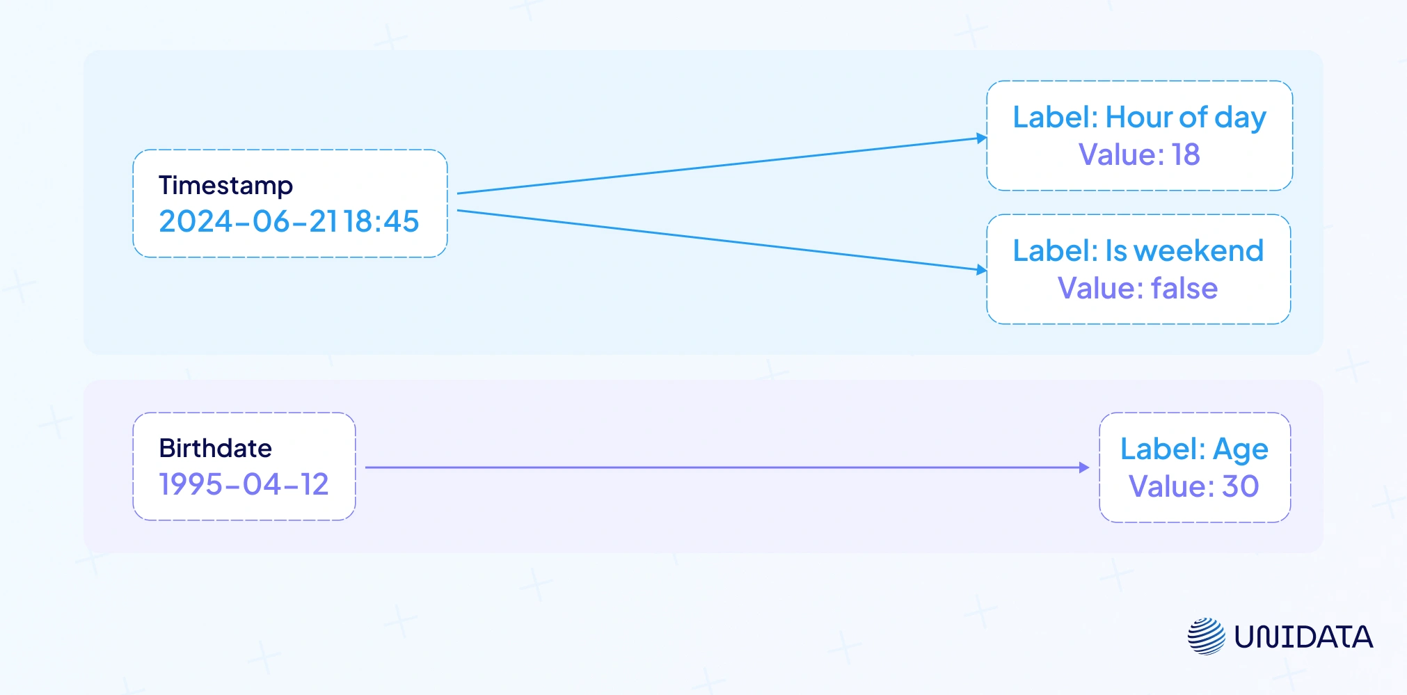
Feature creation is where data scientists turn raw data into new features a model can actually learn from. A timestamp becomes “hour of day” or “is_weekend.” A birthdate becomes “age.” These input data features reveal hidden patterns that machine learning models use for accurate predictions.
Analysts note that creation often means splitting, binning, or one-hot encoding. From relational data, you might build “total purchases in 30 days.” In text, you add word counts; in time-series, lag values or moving averages. Sometimes tools handle it — automated feature engineering can churn out thousands of feature vectors in minutes.
On Kaggle, entire leaderboards have flipped when winners dropped in thousands of crafted model features built from logs and summaries. The payoff is clear: good feature creation feeds your model signal it would never see on its own.
You derived new features from existing fields. Here’s that in code: split time, build ratios, add simple aggregates:
import pandas as pd

# Assume df has: user_id, timestamp, amount, income, cost
df["ts"] = pd.to_datetime(df["timestamp"])

# 1) From timestamp → discrete features
df["hour"]  = df["ts"].dt.hour
df["dow"]   = df["ts"].dt.dayofweek
df["month"] = df["ts"].dt.month

# 2) Mathematical combinations (ratios / interactions)
df["margin"] = (df["income"] - df["cost"]).clip(lower=0)
df["roi"]    = (df["income"] / df["cost"]).replace([pd.NA, pd.NaT], 0).fillna(0)

# 3) Simple relational-style aggregate (user behavior)
df = df.sort_values("ts")
df["amt_7d_sum"] = (
    df.set_index("ts")
      .groupby("user_id")["amount"]
      .rolling("7D").sum()
      .reset_index(level=0, drop=True)
      .fillna(0)
)
Feature Extraction: Distilling Information from Data
Feature extraction is like reducing a long novel to key quotes. You keep the essence. You cut noise. The goal is simple. Turn many inputs into compact feature vectors. Capture structure in fewer dimensions.
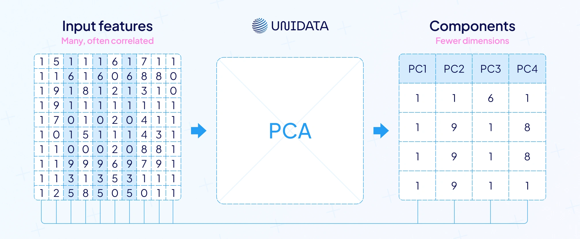
The classics first. PCA squeezes correlated features into a few components. They are abstract. They keep the most variance. LDA does a similar trick. It maximizes class separation. That helps classification. Both speed model training. Both reduce overfitting.
This shines with high-dimensional data. In vision, SIFT and HOG pulled edges and textures. That was before deep learning. In NLP, bag-of-words and TF-IDF still work well. Today, early neural network layers learn features automatically. They spot shapes or phrases.
For tabular data, use modern tools. Autoencoders compress inputs through a bottleneck. Embeddings map high-cardinality categorical features to dense vectors. They replace thousands of one-hot columns. Models handle these compact feature vectors better.
The payoff is clear. You reduce redundancy. You highlight structure. You surface relevant features. Extraction cuts size and noise. It also boosts model performance. Pair it with feature selection next. Extraction builds combined features. Selection keeps the best.
You compress many inputs into a few components while keeping signal. PCA shows the effect:
from sklearn.decomposition import PCA
from sklearn.preprocessing import StandardScaler
from sklearn.pipeline import make_pipeline

num_cols = ["x1","x2","x3","x4","x5"]   # numeric block to compress
pca = make_pipeline(StandardScaler(), PCA(n_components=2, random_state=42))
X_pca = pca.fit_transform(df[num_cols])  # shape: (n_rows, 2) → distilled features
Feature Selection: Picking the Most Relevant Features
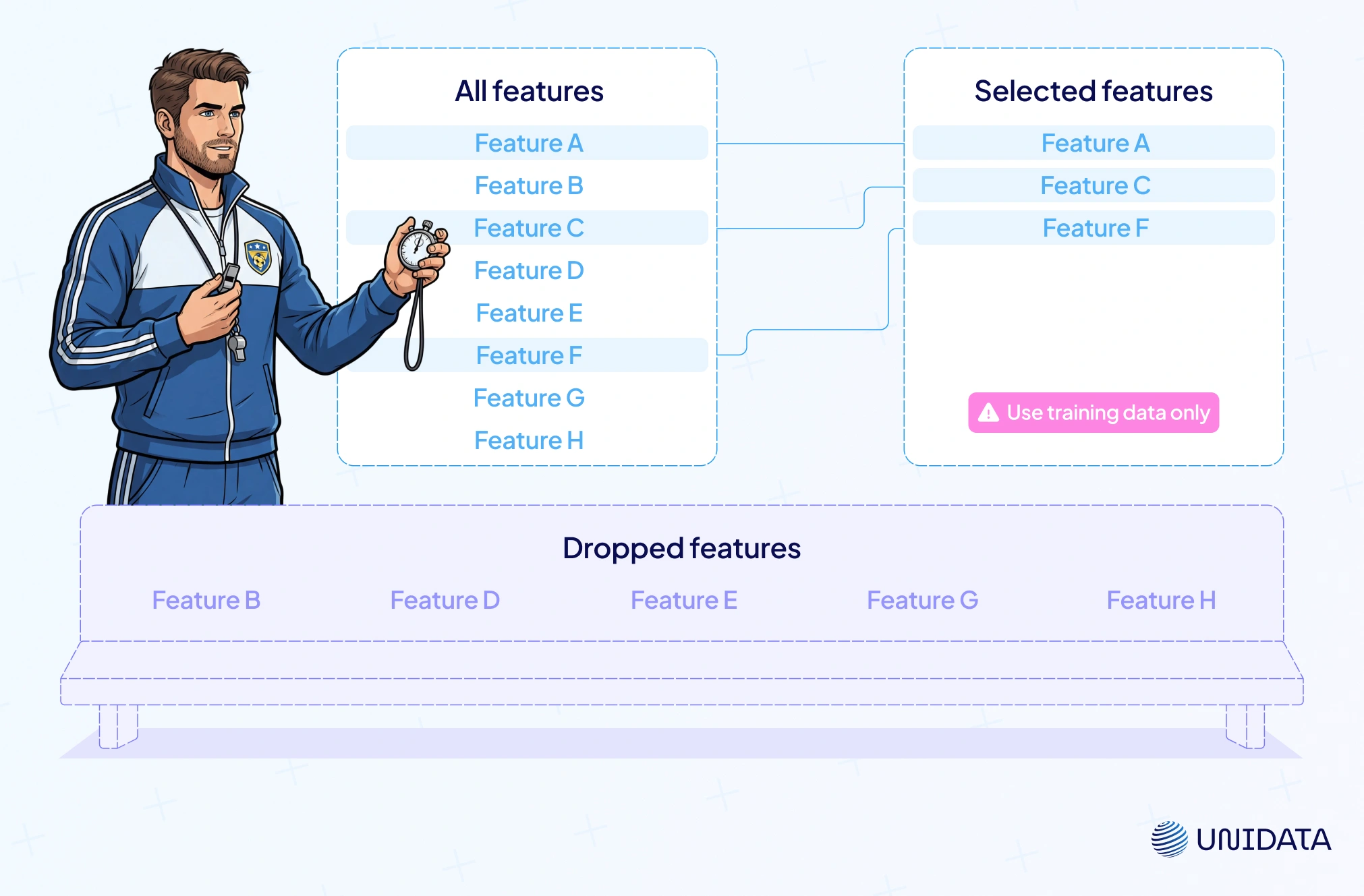
Feature selection is spring cleaning for data. You keep what matters. You toss what doesn’t. Instead of inventing new features, you trim the list to the most relevant features. The payoff is a simpler model, less overfitting, and often sharper model accuracy.
Think of it as building a sports team. You start with a roster of players. You pick the MVPs. You bench the weak links. Too many irrelevant model features slow learning and confuse the algorithm. By narrowing to a lean set, you cut dimensionality and let the model focus on signal, not noise.
There are three main techniques:
- Filter methods. Rank features by correlation or mutual information with the target. Keep the high scorers. Fast, but treats features one by one.
- Wrapper methods. Train and test subsets directly. Use recursive feature elimination to drop the weakest, or forward selection to add the strongest. Precise but costly.
- Embedded methods. Some algorithms do the pruning inside training. L1 (Lasso) regression sets weights to zero. Trees and ensembles output importance scores that reveal which features matter.
The benefits go beyond accuracy. A smaller set of data features means faster training and simpler interpretation. In healthcare or finance, this transparency is vital. With limited samples, like in genomics or IoT, trimming helps avoid overfitting.
A warning though: never peek at test data. Select features only from training data. In time series, don’t use future info. Done right, feature selection surfaces the most relevant information with minimal complexity. You keep only the most relevant features. Here’s filter + model-based selection in a few lines:
from sklearn.feature_selection import mutual_info_classif, SelectFromModel
from sklearn.linear_model import LogisticRegression
from sklearn.preprocessing import StandardScaler
from sklearn.pipeline import make_pipeline
import numpy as np

feat_cols = [c for c in df.columns if c not in ["target","timestamp","ts"]]

# 1) Filter: rank by mutual information
mi = mutual_info_classif(df[feat_cols], df["target"], random_state=42)
top_feats = [f for f, _ in sorted(zip(feat_cols, mi), key=lambda z: z[1], reverse=True)[:20]]

# 2) Embedded: sparse weights select features
sel = SelectFromModel(LogisticRegression(penalty="l1", solver="liblinear", random_state=42))
sel.fit(StandardScaler().fit_transform(df[top_feats]), df["target"])
selected = [f for f, keep in zip(top_feats, sel.get_support()) if keep]
Feature Transformation: Converting Data for Better Understanding
Feature transformation changes form, not meaning. You reshape raw data features so machine learning algorithms can use them. The aim is simple: make inputs machine-readable and boost model performance.
Start with categories
One-hot encoding turns categorical data into binary columns, keeping labels separate with no fake order. If the data is ordinal (S < M < L), use an ordered mapping instead. Numbers can move the other way too. Binning groups a continuous variable (e.g., age → 0–18, 19–35, 36–50). That reduces noise and captures non-linear effects.
Add core transforms
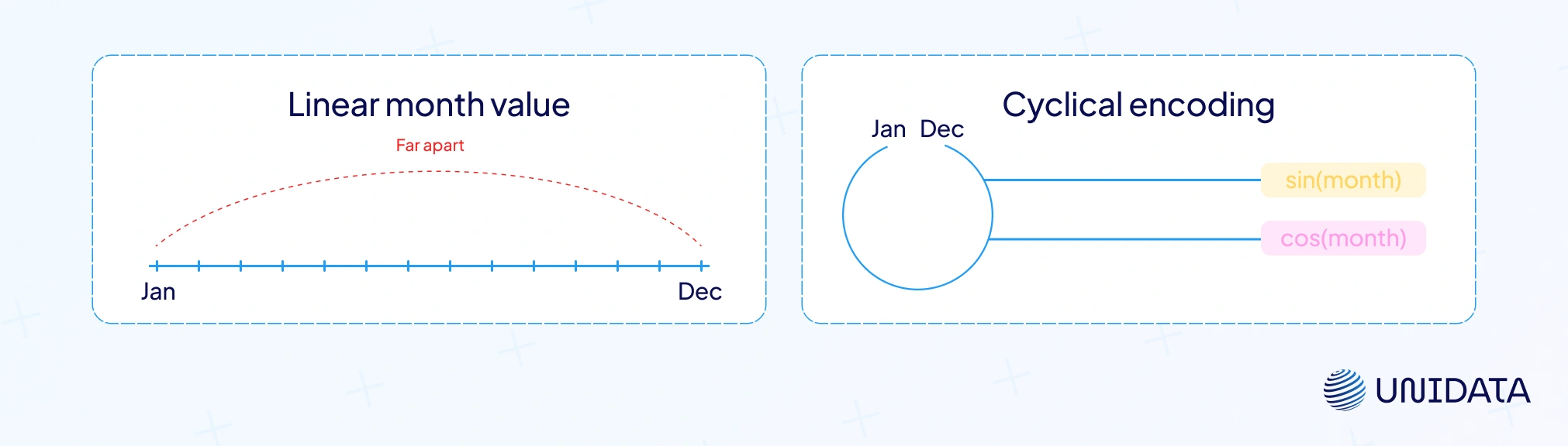
Scaling and normalization align ranges so one large-scale feature doesn’t dominate. Power transforms (log, sqrt, Box-Cox) tame skew and stabilize variance. Polynomial/interaction terms (X², X×Y) let linear models learn curves. For high-cardinality categorical features, try target or frequency encoding, or dense embeddings learned by neural networks. For cyclical fields (hour, month), use sine/cosine so December sits next to January.
Why it matters
Same information, better shape. A network can read pixels as 0–255, but normalizing to 0–1 makes model training steadier and improves model accuracy.
You reshape features (same meaning, better form): encode categories, bin numbers, add cyclical time:
import numpy as np
from sklearn.preprocessing import OneHotEncoder
import pandas as pd

# 1) One-hot for nominal categories
ohe = OneHotEncoder(handle_unknown="ignore", sparse_output=False)
city_ohe = ohe.fit_transform(df[["city"]])                 # → binary columns
city_cols = [f"city_{c}" for c in ohe.categories_[0]]
city_df = pd.DataFrame(city_ohe, columns=city_cols, index=df.index)

# 2) Binning a continuous variable
df["age_bin"] = pd.cut(df["age"], bins=[0,18,35,50,120], labels=["0-18","19-35","36-50","50+"])

# 3) Cyclical encoding for hour
df["hour_sin"] = np.sin(2*np.pi*df["hour"]/24)
df["hour_cos"] = np.cos(2*np.pi*df["hour"]/24)

# Combine back if needed
df = pd.concat([df.drop(columns=["city"]), city_df], axis=1)
Feature Scaling: Normalizing for Fair Comparisons
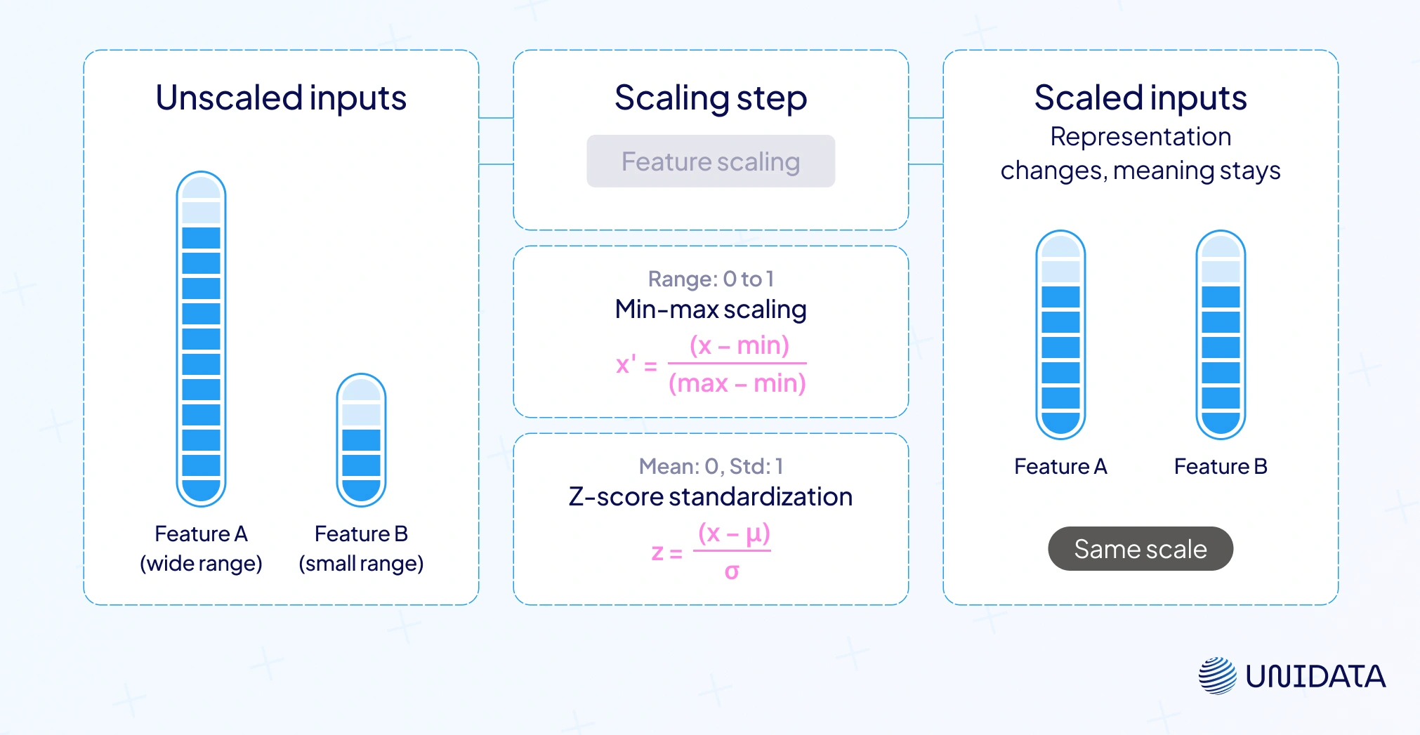
Unscaled inputs skew learning. A wide-range field drowns a tiny one. Feature scaling fixes that. It standardizes ranges so machine learning algorithms compare features fairly. Two core options:
Min-max scaling
Rescale to 0–1 with:
$$ x' = \frac{x - x_{\min}}{x_{\max} - x_{\min}} $$Fast. Precise bounds. Sensitive to outliers.
Z-score standardization
Center to mean 0, std 1 with:
$$ z = \frac{x - \mu}{\sigma} $$Stable for PCA, linear models, and neural networks that use gradient descent.
There are variants. Robust scaling uses medians and IQR to resist outliers. Clipping tames extremes before scaling. Scale first for distance-based methods (KNN, K-Means) and any optimizer that’s touchy about step sizes. Skip for most tree models, but keep pipelines consistent (one transform path for training data and production).
Why Feature Engineering Matters for Model Accuracy
Great inputs beat great tuning. On structured data, good feature engineering turns raw data into relevant features. Machine learning models learn faster. Model accuracy and model performance go up.
What changes when you engineer features
- More signal, less noise. Add season flags. Add time-since-event. Clean categorical features with one-hot encoding.
- Stability. Fewer spurious links. Clearer logic. Easier to explain.
| Cause | Typical move |
|---|---|
| Add clear signal | Add seasonality, recency, clean encodings |
| Remove redundancy | Drop collinear fields; select by mutual information |
| Focus on what matters | Prune with tree importance scores; combine weak fields |
| Use human insight | Ratios (e.g., spend/income), domain flags |
Key Feature Engineering Techniques and Tips
Real datasets are rarely clean. They come with gaps, mixed types, and messy distributions. This is where the toolbox of feature engineering techniques helps turn raw data into relevant features that boost model accuracy.
Imputation of Missing Values
Every dataset has holes. How you fill them changes what the model learns. Numbers often take a mean or median. Categories get a mode. Sometimes the gap itself is signal, so add a “was_missing” flag. For trickier cases, fit a light model to predict the missing. Whatever you choose, keep it consistent across training data and inference scikit-learn.
Encoding Categorical Variables
Models need numbers, not labels. One-hot encoding works for small sets. Ordered groups like “low–medium–high” deserve ordinal scales. Huge cardinality calls for target or frequency encoding, hashing, or embeddings. Rare categories? Collapse them into “Other.” Done right, this step turns messy categorical features into clean feature vectors.
Feature Scaling and Normalization
Scale matters. A large-range feature can drown out the rest. Min–max scaling locks values into [0,1]. Z-score puts features around 0 with unit variance. Robust scaling keeps outliers in check. Use scaling for distance-based algorithms and PCA; tree models usually don’t care scikit-learn.
Interaction Features
Some signals only show up when features meet. Ratios like spend ÷ income. Products like age × income. Powers like X². These help linear models catch curves and context. Generate freely, but prune ruthlessly using validation scores or mutual information.
Time-Based Features
Timestamps are gold. Break them into hour, weekday, or month to reveal cycles. Add lags and rolling averages for trend and momentum. Features like “time since last event” are often game changers in churn or fraud tasks. For cyclical values, sine and cosine keep December next to January where it belongs pandas.
Aggregations in Relational Data
Multi-table data needs summaries. Count purchases in 30 days. Track average basket size. Capture unique logins. These roll-ups give models instant context. Many teams store them in a feature store for reuse and consistency.
Dimensionality Reduction
Too many features add noise. PCA reduces correlated inputs to a few components. Autoencoders compress data into dense codes. Embeddings turn sprawling categorical sets into compact numeric space. The point is simple: fewer inputs, same signal.
Feature Selection
After creation comes pruning. Filters rank by correlation, variance, or mutual information. Wrappers test subsets with recursive elimination or forward selection. Embedded methods like Lasso or decision trees bake selection into training.
Iterative Refinement
This is never one-and-done. Feature engineering is an iterative process. Plot distributions. Inspect errors. Drop, reshape, or invent features until validation improves. Each round is a new question to the data. Over time, you build instinct about what works IBM.
The Feature Engineering Process (From Raw Data to Model)
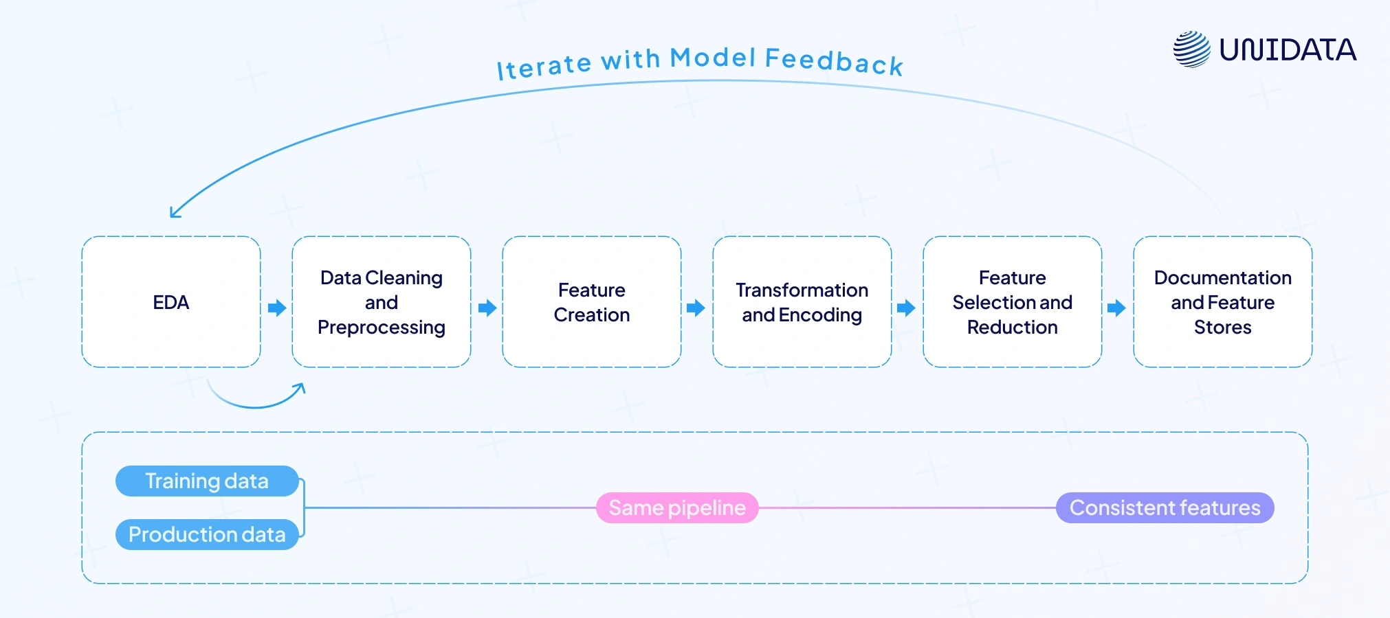
Feature engineering is rarely a straight line. It’s more like shaping clay — analyze, mold, reshape, and refine until the features fit the model. Here’s how the process usually flows.
- Exploratory Data Analysis (EDA)
Start by looking, not building. Plot distributions. Check correlations. Scan records. Spot outliers and missing values. EDA shows which raw features might need a log transform, binning, or encoding. It also hints at which ones carry little signal.
- Data Cleaning and Preprocessing
This is washing your ingredients before cooking. Handle missing values, fix types, and remove duplicates. Cap or transform outliers. Standardize formats like time zones or text. Models are sensitive to “garbage in,” so this step directly affects downstream model accuracy.
- Feature Brainstorming and Creation
Now the creative phase. Use domain knowledge to dream up ratios, flags, or group stats. Pull in external data if allowed. Start simple, then stack complexity. Create → test → refine. Keep notes on what each feature means; you’ll thank yourself later.
- Transformation and Encoding
Once created, features must be model-friendly. Encode categorical variables with one-hot or target encoding. Scale numbers where needed. Bin continuous values if categories work better. Automate in a pipeline so the same logic applies to training, validation, and production scikit-learn.
- Feature Selection and Reduction
Too many features can blur the picture. Use correlation, mutual information, or model-based importance scores to prune. Quick baseline models help reveal which features matter. Watch for leakage — a suspiciously strong feature may just be a proxy for the target.
- Iteration with Model Feedback
Train, test, adjust. If accuracy lags, study errors. Maybe a subgroup underperforms — add a feature to capture it. Maybe an expected feature underdelivers — try a new encoding. This loop is the heart of the feature engineering process, and top Kaggle teams may run through it hundreds of times.
- Documentation and Feature Stores
Final features should be reusable. Production teams log them in a feature store, a centralized hub for storing definitions and computations Google Feature Store. This avoids “lab vs. production” mismatches and keeps features consistent across models.
Automated Feature Engineering and Tools
Manual feature work is powerful, but slow. That’s why automated feature engineering (AFE) has emerged — to let machines handle the routine, while humans focus on insight. No tool fully replaces a data scientist, but the right ones can cut weeks of work into hours.
Feature synthesis libraries

Tools like FeatureTools or tsfresh generate hundreds of candidate features automatically. They combine relational tables, run aggregations, and output features such as “average spend in last 7 days.” What once took a Kaggle team days of GPU crunching can now be done in minutes.
AutoML platforms

Systems such as Google AutoML Tables or H2O Driverless AI fold feature generation into their pipelines. They test encodings, log transforms, bins, and interactions as part of model search. The upside: surprising new features. The risk: computational cost and meaningless combos if left unchecked.
Generative AI helpers
Large language models are starting to suggest or even code feature ideas. Early research shows LLMs can propose useful transformations or write pandas snippets. Human oversight is still vital to prevent leakage or nonsensical features, but this space is moving fast.
Conclusion
Feature engineering is the lever that moves results. You turn raw data into relevant features through feature creation, feature extraction, feature selection, feature transformation, and feature scaling. That shift lifts model accuracy and stabilizes model performance across real training data and live machine learning pipelines. Do this well and models learn faster, generalize better, and explain themselves.