Learn what outliers are, why they can wreak havoc in your data analysis, how to spot them visually & statistically, and strategies to handle them effectively.
Ever had that one weird data point ruining your perfect analysis? It’s the statistical equivalent of a party crasher – an outlier. Don’t worry, every data scientist deals with them. We’re here to help you spot these troublemakers and decide what to do next (even if that means keeping a few).
What Exactly Is an Outlier?

An outlier is a data point that doesn’t fit with the rest of the data set. Formally, it’s an observation lying an abnormal distance from other values. In plain words: it’s that unusual data point that makes you stop and ask, “Is this value real?”
These rare cases are also called anomalies in machine learning and data analysis. Outlier identification isn’t always clear-cut — context decides what’s truly “abnormal” NIST.
Why do they occur? Sometimes by chance — any distribution can produce extreme values. Other times, they flag data entry errors, measurement errors, or mixing in a different population IBM. For instance, a sudden 1,000 °C spike in a temperature log or an extra zero in a financial record would both qualify as outliers. Outliers may also signal a heavy-tailed distribution, where unusual data points are naturally more common.
Outliers come in two main types: mild outliers (slightly outside the pack) and extreme outliers (far away). You’ll also hear about high outliers and low outliers, depending on whether the value lies unusually high or unusually low. No matter the flavor, outliers can heavily influence your data analysis.
Why Do Outliers Matter?
Outliers can wreak havoc on your analysis. They pull results in their direction like a magnet. A single extreme value can distort the mean and standard deviation.
Statistical methods from regression to PCA are sensitive to them NIST. In regression, one point can tilt the line, shift coefficients, and flip p values. Such points are called influential observations. Just one or two can change your model’s story.
Outliers also disrupt forecasts. Imagine web traffic spiking 10× in one day — the overall trend looks nothing like reality. Machine learning models suffer too. Distance-based methods may treat an outlier as its own cluster. Regression can twist to fit that weird point. Even the z score method misfires because the inflated standard deviation hides how many standard deviations away the point really is.
But outliers aren’t always bad. In fraud detection, they are the signal. In science, an unusual data point might reveal a breakthrough. As NIST notes, outliers can highlight data entry errors, unexpected effects, or even rare new patterns NIST.
In short: outliers matter because they distort results, reduce generalizability, and risk wrong conclusions. Yet deleting them blindly can throw away valuable insight. The challenge is deciding when an outlier is noise — and when it’s the clue you’re looking for.
How to Spot Outliers
Finding outliers is part art, part science. There are two main approaches: visual detection with plots and statistical detection with formulas or tests NIST. Often, you’ll use both for a complete sweep of your data set.
Visual Methods: Scatter Plots, Histograms, and Box-and-Whisker Plots
Visualizing your data is the fastest way to spot outliers. As the saying goes, “plot your data before you trot your data.” Two of the most useful charts are the scatter plot and the box-and-whisker plot NIST.
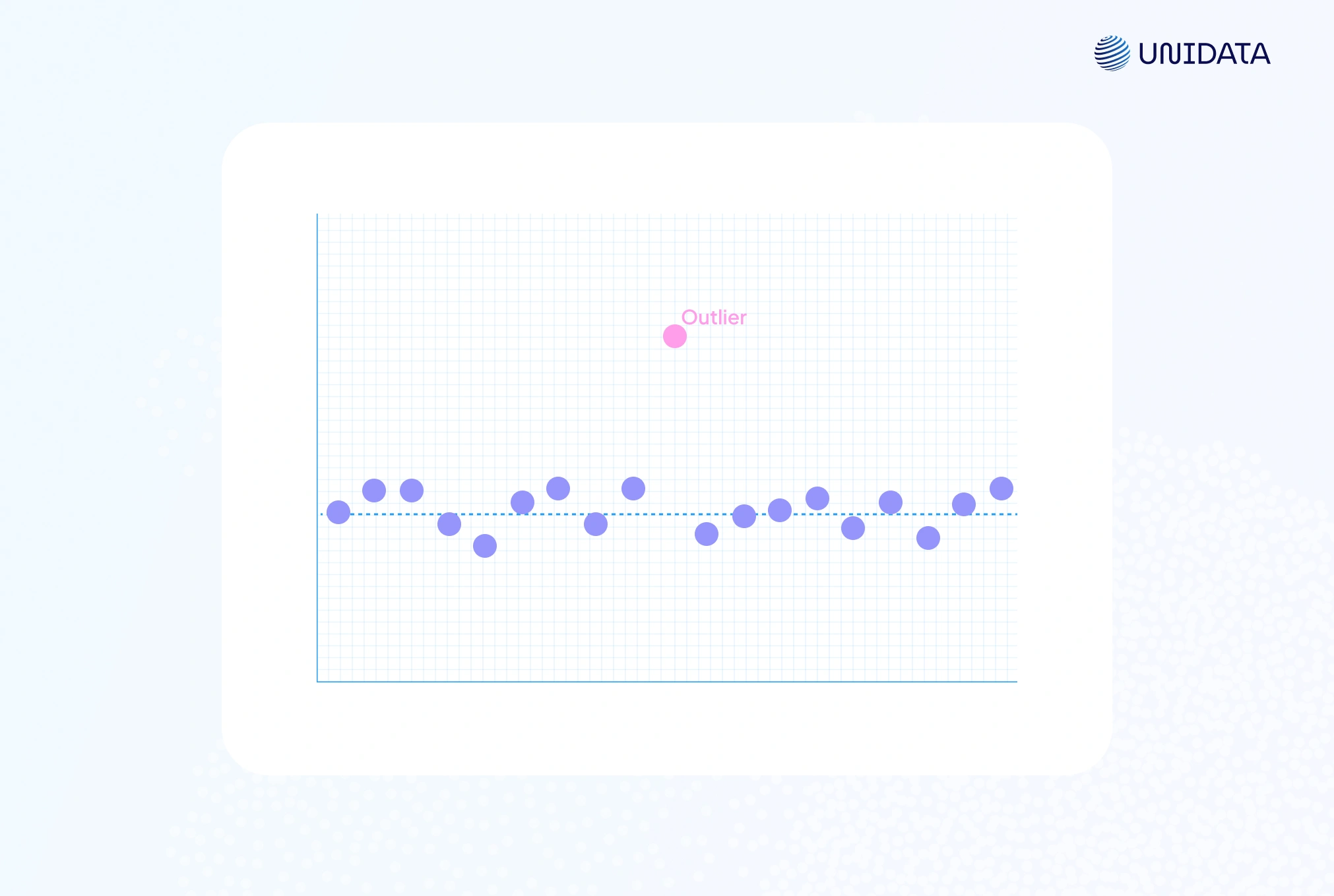
A scatter plot highlights outliers as points far from the main cluster. For instance, a single red dot high above the rest is a clear high outlier. These plots are especially useful for two variables, where one point breaks the Y–X trend.
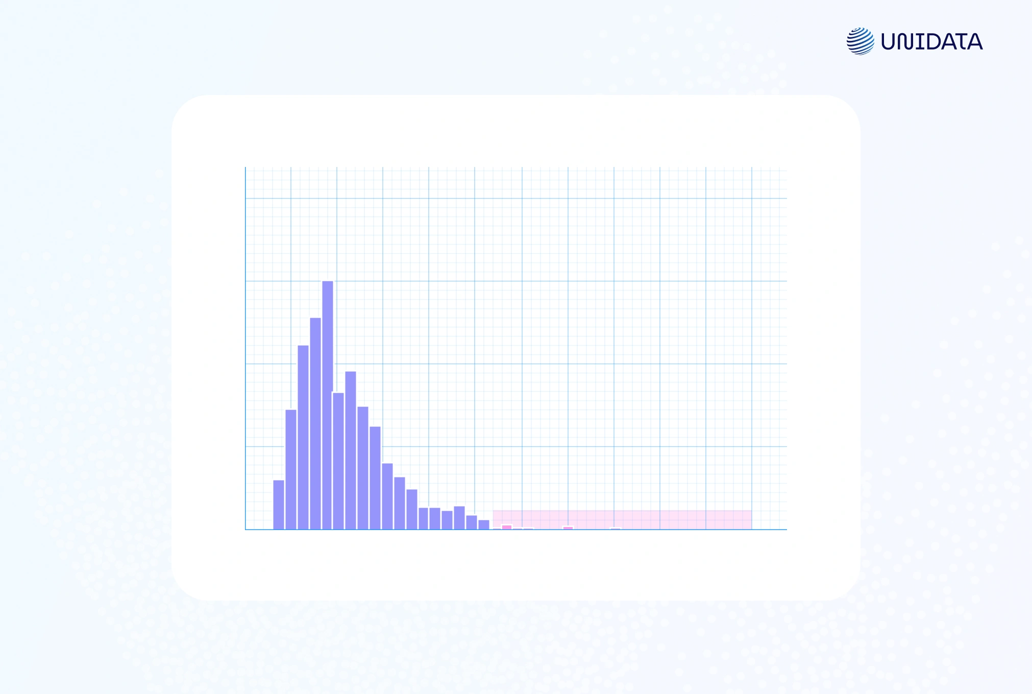
A histogram can also expose unusual data points. Most values fill a few bins, while an isolated bar at the edge signals an outlier.
The box-and-whisker plot (or box plot) is often the MVP. It shows the median, the first quartile (Q1), the third quartile (Q3), and flags potential outliers using the IQR method. Whiskers extend to 1.5 × IQR, and any data point beyond is plotted separately NIST. For example, a red dot beyond the whisker clearly marks an extreme case.
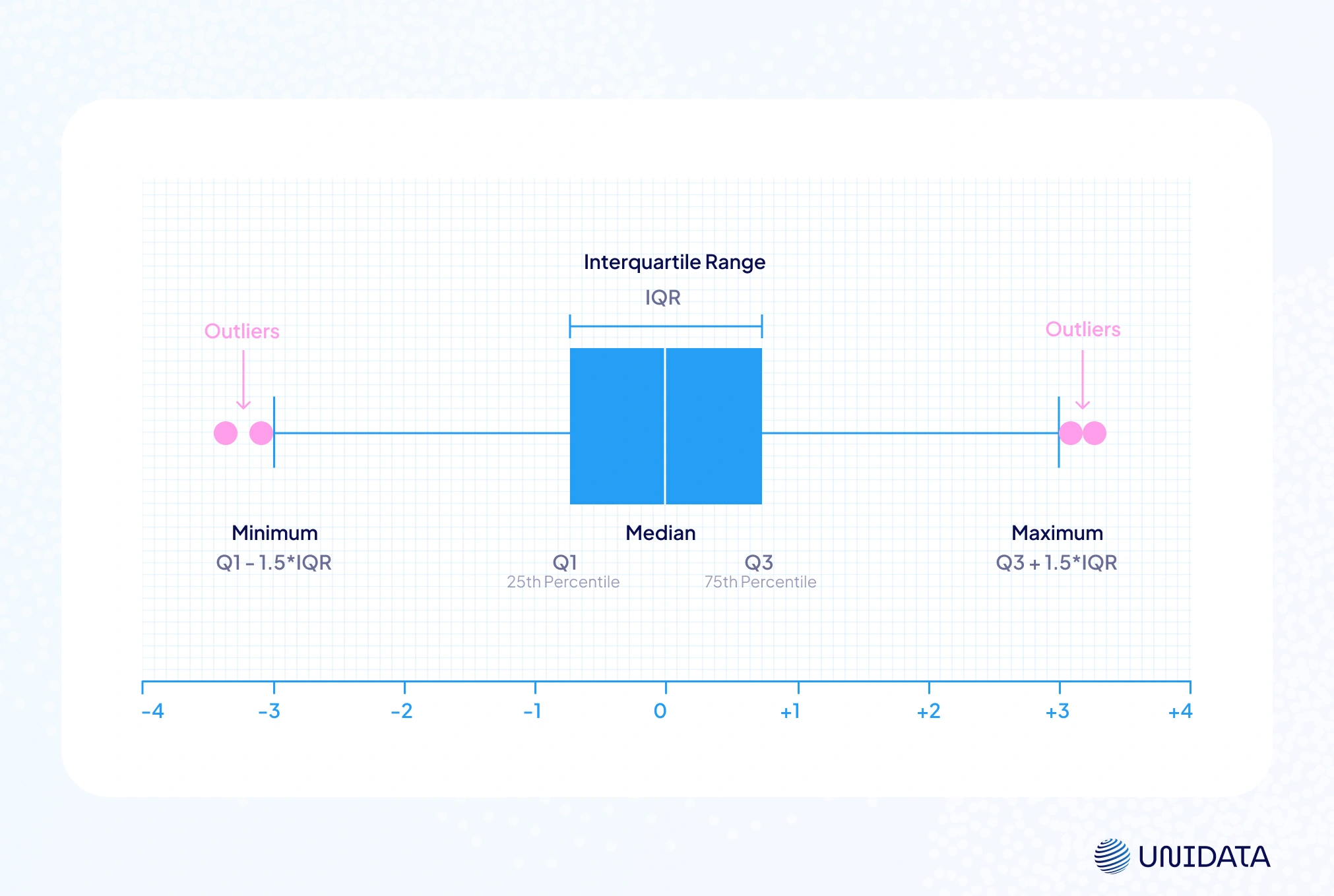
By convention, any point above the upper fence or below the lower fence is flagged. This makes box plots a hybrid of visualization and rule-based outlier detection. One chart shows both the distribution and which points may be troublemakers.
Visual methods are intuitive and quick. You can often identify outliers at a glance, and even see context — like if they cluster on a certain day or in a category. But they’re subjective and don’t scale well in high dimensions. That’s where statistical methods come in.
Python Example
Here’s how you can quickly visualize outliers in Python using Matplotlib. We’ll create a simple dataset and plot it:
import numpy as np
import matplotlib.pyplot as plt

# Sample data: 100 points around 50 plus one extreme outlier at 100
np.random.seed(42)
data = np.concatenate([np.random.normal(50, 5, size=100), [100]])

# Scatter plot
plt.figure(figsize=(5, 3))
plt.scatter(range(len(data)), data, color='steelblue')
plt.axhline(np.mean(data), color='green', linestyle='--', label='Mean')
plt.scatter(len(data)-1, data[-1], color='red', label='Outlier')  # highlight the outlier
plt.title("Scatter Plot with Outlier")
plt.xlabel("Index"); plt.ylabel("Value")
plt.legend(); plt.show()

# Box plot
plt.figure(figsize=(5, 1.5))
plt.boxplot(data, vert=False, flierprops={'markerfacecolor':'red', 'marker':'o'})
plt.title("Box Plot of Values")
plt.xlabel("Value")
plt.show()
This code draws a scatter plot and a box-and-whisker plot. In the scatter plot, the outlier shows up as a red point far above the main cluster. In the box plot, it appears as a red marker beyond the whiskers, making the unusual data point easy to spot.
The Interquartile Range (IQR) Method
A classic tool for outlier detection is Tukey’s IQR method. It’s simple, non-parametric, and works well for one-dimensional data NIST.
First, calculate the interquartile range (IQR):
$$\text{IQR} = Q_3 - Q_1$$where Q1 is the first quartile (25th percentile) and Q3 is the third quartile (75th percentile). For instance, if Q1 = 10 and Q3 = 20, then IQR = 10. The IQR measures the spread of the middle 50% of your data set.
Next, set the fences:
- $\text{Lower\ Fence} = Q_1 - 1.5 \times \text{IQR}$
- $\text{Upper\ Fence} = Q3 + 1.5 \times \text{IQR}$
Some analysts also use 3 × IQR for “extreme values”. Any data point outside these ranges is flagged as a potential outlier. Those just beyond 1.5 × IQR are “mild” outliers, while those beyond 3 × IQR are “extreme outliers.”
For instance, if Q1 = 5 and Q3 = 15, IQR = 10. The fences are −10 and 30. A point at 42 lies above 30 and is an outlier. A point at 29 is inside the fence and not flagged.
Why 1.5 × IQR? The cutoff is arbitrary but practical. It balances sensitivity without over-flagging. Because the method uses medians and quartiles, it’s robust — unlike the mean and standard deviation, it isn’t pulled around by a single high outlier.
The IQR method works best for univariate data. It doesn’t assume a normal distribution, so it handles skewed data well. If the data are normal, 1.5 × IQR corresponds to roughly ±2.7σ. Only about 0.7% of values fall beyond that, so the rule makes intuitive sense.
Python Example – IQR Method
Here’s how to flag outliers in Python:
import numpy as np

# Suppose data is a 1D NumPy array
Q1 = np.percentile(data, 25)
Q3 = np.percentile(data, 75)
IQR = Q3 - Q1
lower_fence = Q1 - 1.5 * IQR
upper_fence = Q3 + 1.5 * IQR

outliers = [x for x in data if x < lower_fence or x > upper_fence]
print("IQR method outliers:", outliers)
This prints any values outside the 1.5 × IQR fences. It’s just a few lines of code. In pandas, you can do the same with: df[(df[col] < lower_fence) | (df[col] > upper_fence)]
Pros & Cons: The IQR method is simple, robust, and built into box plots. Because it uses medians, it’s not distorted by extreme values. But it can over-flag points in heavy-tailed distributions, where frequent mild outliers are normal IBM. Another limitation: it only works on one variable at a time. To catch unusual combos across variables, you need multivariate methods like Mahalanobis distance.
Z-Score Method (Standard Deviation Method)
Another common way to identify outliers is with the z score. It measures how many standard deviations a data point is from the mean.
The formula is:
$$z = \frac{x - \mu}{\sigma}$$where μ is the mean and σ is the standard deviation of the data set. If the absolute value of $z$ is greater than 3, the point is flagged as an outlier. This is the classic ±3σ rule. In a normal distribution, about 99.7% of values fall within ±3σ, so anything beyond is rare.
For instance, if the mean is 100 and σ = 10:
- X = 140 → z = +4.0 → four standard deviations away → flagged as an outlier.
- X = 85 → z = −1.5 → within 3σ → not an outlier.
The z score method is easy to compute. SciPy provides scipy.stats.zscore() to calculate z-scores for an array docs.scipy.org. You can also implement it manually or use pandas to standardize a column.
Python Example – Z-Score
Using the same data array as before:
from scipy import stats

z_scores = stats.zscore(data)
# Get indices of points with |z| > 3
outlier_indices = np.where(np.abs(z_scores) > 3)
print("Z-score outlier values:", data[outlier_indices])
This code prints values with a z score above 3 or below −3. (The data set should be roughly normal for this rule to apply.) If the distribution isn’t normal, ±3 may be too strict or too loose. Some fields use ±2.5 or ±3.5, but ±3 is the classic cutoff.
Pros & Cons
The z score method is easy, parametric, and widely used — “>3 standard deviations = outlier” is a common rule. But in heavy-tailed distributions, the mean and standard deviation get distorted by extreme values, leading to too many or too few flagged points. Like the IQR method, it’s univariate and can miss unusual combos across features. A robust alternative (e.g., median absolute deviation) helps, but in practice, z-scores work best for bell-shaped data without heavy skew.
Grubbs’ Test (Statistical Test for Outliers)
Unlike the IQR method or the z score method, Grubbs’ test is a formal hypothesis test for outlier detection. It assumes normality and is especially useful with small data sets.
The null hypothesis (H₀) states “no outliers.” The test statistic is:
$$ G = \frac{\max\!\left|\,Y_i - \bar{Y}\,\right|}{s} $$where Ȳ is the mean and s is the standard deviation.
This is basically the largest absolute z score. If G exceeds the critical value from the t-distribution, the most extreme value is a statistically significant outlier.
Grubbs’ test finds one outlier at a time. For multiple outliers, extensions like Tietjen-Moore or Generalized ESD are recommended.
It’s often used in chemistry, engineering, and lab work where data integrity is strict. For example, if you have ten measurements and one looks far off, Grubbs’ test helps decide if it’s random variation or a true outlier.
Python Example – Grubbs’ Test
!pip install outliers  # ensure the outliers package is installed
from outliers import smirnov_grubbs as grubbs

# Two-sided Grubbs' test (detects highest or lowest outlier)
result = grubbs.test(data, alpha=0.05)
print("Data after Grubbs' test:", result)
This code removes the most extreme value at 5% significance and returns the trimmed data set. You can also run grubbs.max_test or grubbs.min_test to check the highest or lowest point. If no outlier is found, the data is unchanged.
Grubbs’ test is powerful for small samples, offering a p value to guide decisions. It gives a formal, quantitative rule — useful in reports or publications.
Pros & Cons: Rigorous and statistically sound, but assumes a normal distribution, detects only one outlier at a time, and can over-flag in very large data sets. As IBM notes, removing outliers is controversial, so always combine the test with domain knowledge.
Mahalanobis Distance (Multivariate Outliers)
So far, we’ve looked at outlier detection one feature at a time. But a data point can look normal in each feature yet still be unusual in combination. That’s where Mahalanobis distance comes in.
It’s essentially a multivariate z score. For a vector x, the distance from the mean vector μ is:
$$D_M(x) = (x - \mu)^{T} \Sigma^{-1} (x - \mu)$$where Σ⁻¹ is the inverse covariance matrix.
This accounts for correlations — shrinking distances along correlated directions and emphasizing the unusual ones.
If the data set is approximately multivariate normal, squared distances follow a chi-square distribution with p degrees of freedom. A cutoff from the χ² table flags potential outliers.
For example, with two variables, D² > 9.21 is an outlier at ~1% significance.
Use case:
Mahalanobis distance detects outliers in combinations — like someone 6’5” but only 100 lbs. Neither value is extreme alone, but together they are. It’s also widely used in regression diagnostics to find influential observations with high leverage.
Python Example – Mahalanobis Distance
import numpy as np
from numpy.linalg import inv
from scipy.stats import chi2

# Example 2D data (each row is an observation, columns are features)
X = np.array([[1.2, 3.5],
              [2.1, 3.0],
              [0.8, 4.1],
              [2.5, 3.8],
              [10.0, 15.0]])  # last point is an obvious outlier

# Compute mean and covariance
mu = X.mean(axis=0)
cov = np.cov(X, rowvar=False)
inv_cov = inv(cov)

# Compute Mahalanobis distances
distances = []
for x in X:
    diff = x - mu
    dist = np.sqrt(diff.dot(inv_cov).dot(diff))
    distances.append(dist)

# Determine threshold (e.g., 99th percentile for chi-square with df=2)
threshold = np.sqrt(chi2.ppf(0.99, df=X.shape[1]))
outliers = [i for i, d in enumerate(distances) if d > threshold]
print("Mahalanobis distances:", distances)
print("Outlier indices:", outliers)
The code computes Mahalanobis distance for each point and compares it to the 99th percentile of χ² (df = number of features). [10.0, 15.0] is farthest from the mean and flagged as an outlier.
Pros & Cons: Mahalanobis distance is strong for multivariate outlier detection, since it accounts for correlations and scale. It reveals unusual value combinations that IQR or plain z scores miss. But it assumes an ellipsoidal distribution and relies on a stable covariance matrix. In high dimensions, nearly all data points can look like potential outliers. Still, for moderate data sets, it’s one of the most reliable tools, with implementations in scikit-learn’s EllipticEnvelope.
A Quick Comparison of Outlier Detection Methods
Let’s summarize and compare the methods we’ve discussed (IQR, Z-score, Grubbs’ test, Mahalanobis) and their characteristics:
| Method | Use Case | Assumptions | Pros | Cons |
|---|---|---|---|---|
| IQR Method (Tukey) | Univariate; general use | None (non-parametric) | Simple, robust to non-normal data (uses medians); easy to interpret (1.5×IQR rule) | Might flag many points in heavy-tailed data; ignores anything multivariate |
| Z-Score (Std Dev) | Univariate; roughly normal data | Approx. normal distribution | Easy to calculate; widely understood (±3σ rule) | Affected by outliers (mean, σ not robust); not suitable for skewed distributions |
| Grubbs’ Test | Univariate; small samples or formal testing | Normal distribution (for test validity) | Statistically rigorous (provides p-value); justifies outlier removal with significance level | Only detects one outlier at a time; requires normality; not ideal for large datasets (almost any mild outlier can be “significant”) |
| Mahalanobis Distance | Multivariate outliers (multiple features) | Data roughly elliptical (multivariate normal) | Detects unusual combinations of values; accounts for variable correlations; useful in regression (leverage) | Requires computing covariance (needs sufficient data); can break down in high dimensions or non-elliptical data; assumes a single cluster of data |
Each method has its role, and in practice you often combine them. Start with visuals (box plots, scatter plots), then apply the IQR method or z scores for quick checks. Use Grubbs’ test in small data sets, and for high-dimensional data switch to Mahalanobis distance or advanced methods like isolation forests or local outlier factor in scikit-learn.
Now that you can identify outliers, what should you do with them? That brings us to the next big question: how to deal with these pesky points.
How to Deal with Outliers
Outliers can flip your data analysis upside down. Handle them carelessly and you risk bias; ignore them and they can hijack results IBM. The rule of thumb: figure out why a point is strange, and don’t make changes without documenting.
Removing Outliers (Deleting the Points)
When a value is clearly wrong — say, a 1000 °C sensor glitch — dropping it makes sense. Just compare results with and without it so you’re not sweeping problems under the rug.
# Using IQR fences
cleaned_data = data[(data >= lower_fence) & (data <= upper_fence)]

# Using z-scores
cleaned_data = data[np.abs(z_scores) <= 3]

# Pandas DataFrame
df[(df[col] >= lower_fence) & (df[col] <= upper_fence)]
Imputing or Transforming Outliers
Not ready to delete? Impute with the median, winsorize by capping at percentiles, or transform with logs or Box-Cox to shrink the pull of extreme values.
# Winsorizing with pandas
lower_cap = data.quantile(0.05)
upper_cap = data.quantile(0.95)
capped_data = data.clip(lower=lower_cap, upper=upper_cap)
Flagging Outliers (Keeping but Noting Them)
Another path: keep the record but add a flag. That way you can run models with and without the potential outliers, or even treat the flag as a feature.
df['Outlier_flag'] = ((df[col] < lower_fence) | (df[col] >
upper_fence)).astype(int)
When to Keep Outliers (And When Not To)
Keep outliers when they reflect reality — market crashes, rare lab results, niche clusters. Toss them when they’re obvious data entry errors, irrelevant to your scope, or just noise in massive data sets.
Conclusion
Outliers aren’t just oddballs to delete. They can wreck your stats, spotlight errors, or reveal something game-changing. You’ve seen how to spot them — from scatter plots to Grubbs’ test — and how to handle them with removal, imputation, or robust methods.
The key is context. Sometimes you drop them, sometimes you keep them, but you always explain why. Try your analysis both ways if you’re unsure. Transparency builds trust, and thoughtful outlier handling makes your data analysis stronger, whether it’s a simple regression or a machine learning model. Outliers won’t catch you off-guard now — you’ve got the tools to flag them, tame them, or let them stand.