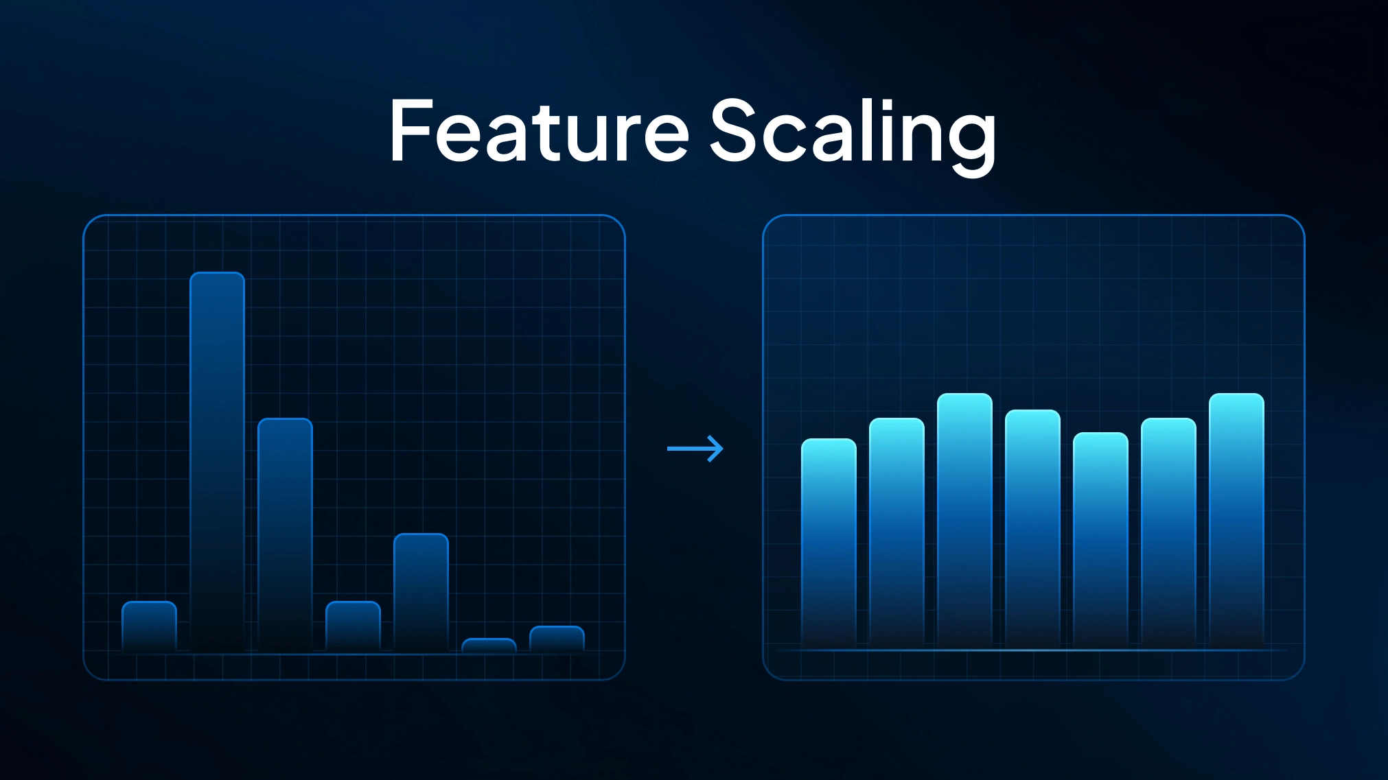
In most datasets, some numbers shout. Others barely whisper. Left unscaled, the louder feature values dominate the model. Feature scaling fixes this. It puts input data on a common scale so all the features contribute equally.
This step in feature engineering looks small but drives big gains. It sharpens distance calculations. It speeds up gradient descent. It keeps results steady across different scales of data. For many machine learning algorithms — from support vector machines to k-means clustering — scaling is the difference between sluggish, skewed learning and crisp, reliable model performance.
What is Feature Scaling and Why Does It Matter?
Feature scaling — or feature normalization — resizes feature values to a common scale. Popular methods include min max scaling into [0,1] and z score normalization with zero mean and unit variance. Without it, a feature measured in thousands, like house price, can drown out another measured in tens, like number of rooms.
Most machine learning algorithms assume all the features contribute equally. On different scales, that balance breaks. Distance based algorithms pick wrong neighbors. Support vector machines misplace margins. Gradient descent slows down instead of converging.
Scaling puts things back in line:
- Boosts accuracy — a scaled SVM leapt from 75 % to 98%; k means clustering also snapped into clearer groups.
- Speeds learning — balanced input data keeps gradient descent steady and fast.
- Adds stability — scaling avoids extreme numbers that break training.
That’s why applying feature scaling is one of the most essential feature engineering techniques in data science. It turns messy raw data into standardized data or normalized values, keeping machine learning models sharp across varying scales.
Impact on Distance-Based Models (k-NN, SVM, k-Means, etc.)
Some machine learning algorithms depend on distance. If features sit on different scales, the math tips over. Feature scaling sets things straight.
- k-NN — Finds the closest data points. But if one feature ranges into the thousands and another into single digits, the wide one always wins. The smaller one is ignored. It’s like letting one friend shout while another whispers — only the loud voice gets heard. With min max scaling or z score normalization, both voices carry. All the features contribute equally.
- k-Means clustering — Splits data into groups. Raw units can confuse it. Dollars, grams, and millimeters don’t line up. The result is messy clusters. Think of trying to sort fruit by both weight and color using different measuring sticks — you end up with odd baskets. After min max or z score normalization, the clusters fall into clear, natural groups.
- Support vector machines — Margins and kernels rely on distances and the dot product. If one input feature runs much larger than the rest, the hyperplane bends out of shape. It’s like a seesaw with one heavy side — balance is gone. With scaling, the seesaw evens out. Accuracy can leap from 75 % to 98 %, with fewer support vectors and cleaner decision boundaries.
Other models — like principal component analysis, regularized regression, and anomaly detection — also work better on a similar scale. Tree-based models and Naive Bayes care less, but scaling rarely hurts.
Common Feature Scaling Techniques (Normalization, Standardization, & More)
Different datasets call for different scaling techniques. The right method depends on the distribution, outliers, and the machine learning algorithm you use. The go-to options are min max normalization, z score normalization, robust scaling, max abs scaling, and log transformation.
Min-Max Normalization (Rescaling to a Range)
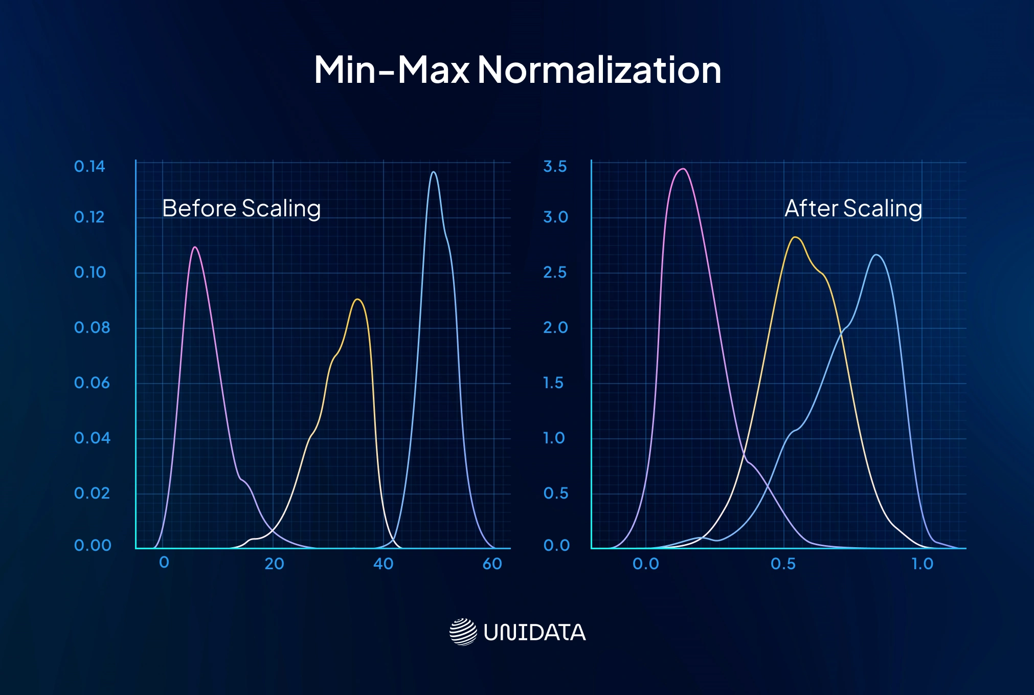
Min max scaling squeezes values into a fixed range — usually [0,1]. Formula:
$$ x_{\text{scaled}} = \frac{x - \min(x)}{\max(x) - \min(x)} $$The smallest becomes 0, the largest 1. Distances between data points stay intact — just compressed.
Where it shines
Neural nets like bounded inputs. Percentages (0–100) and pixel values (0–255) are natural fits. It also makes outputs intuitive — everything becomes a 0–1 score.
The catch
Outliers bend the scale. A single huge maximum value can squash the rest near zero. If you scale before splitting, new testing data may spill outside the original bounds. Always fit on training data first.
Example: Clicks (0–500) and time on site (0–60) sit on different scales. Apply min max normalization. Both now run from 0 to 1, so updates in a neural net stay balanced. If clicks shoot past 500, retrain or cap the scaler.
Z-Score Standardization (Standard Scaler)
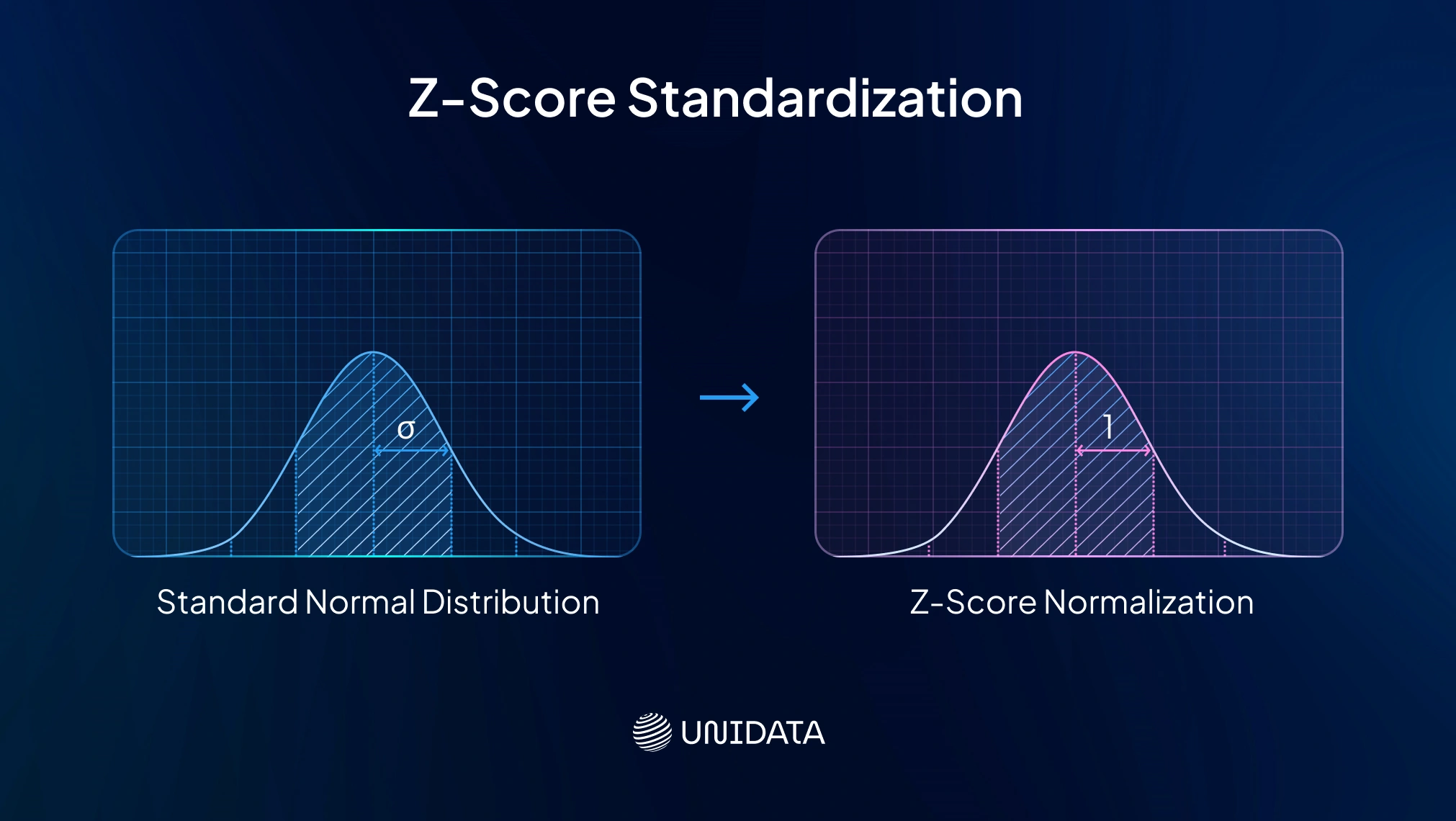
Z score normalization shifts features so their average becomes zero and their spread is measured in standard deviations, giving each feature mean 0 and unit variance. Formula:
$$ x_{\text{scaled}} = \frac{x - \mu}{\sigma} $$Each value is measured in standard deviations from the mean. Think of it like resetting a scoreboard before a new game — everyone starts at zero, no matter their past score.
Use cases
A common default for many machine learning algorithms. Best when data looks roughly Gaussian distribution. Speeds up gradient descent and keeps L1/L2 regularization fair so all the features contribute equally.
Pitfalls
Still sensitive to outliers. A large value can stretch the standard deviation and push other data points toward zero. Also gives no fixed range — values may sit outside [-3,3]. For heavy outliers, robust scaling works better.
Example
Take annual income in thousands and house size in hundreds. Raw numbers sit on different scales. After standardization, both have mean 0 and std 1. A one-unit change equals one standard deviation, so coefficients compare real predictive power, not raw units.
Robust Scaling (Median and IQR Normalization)
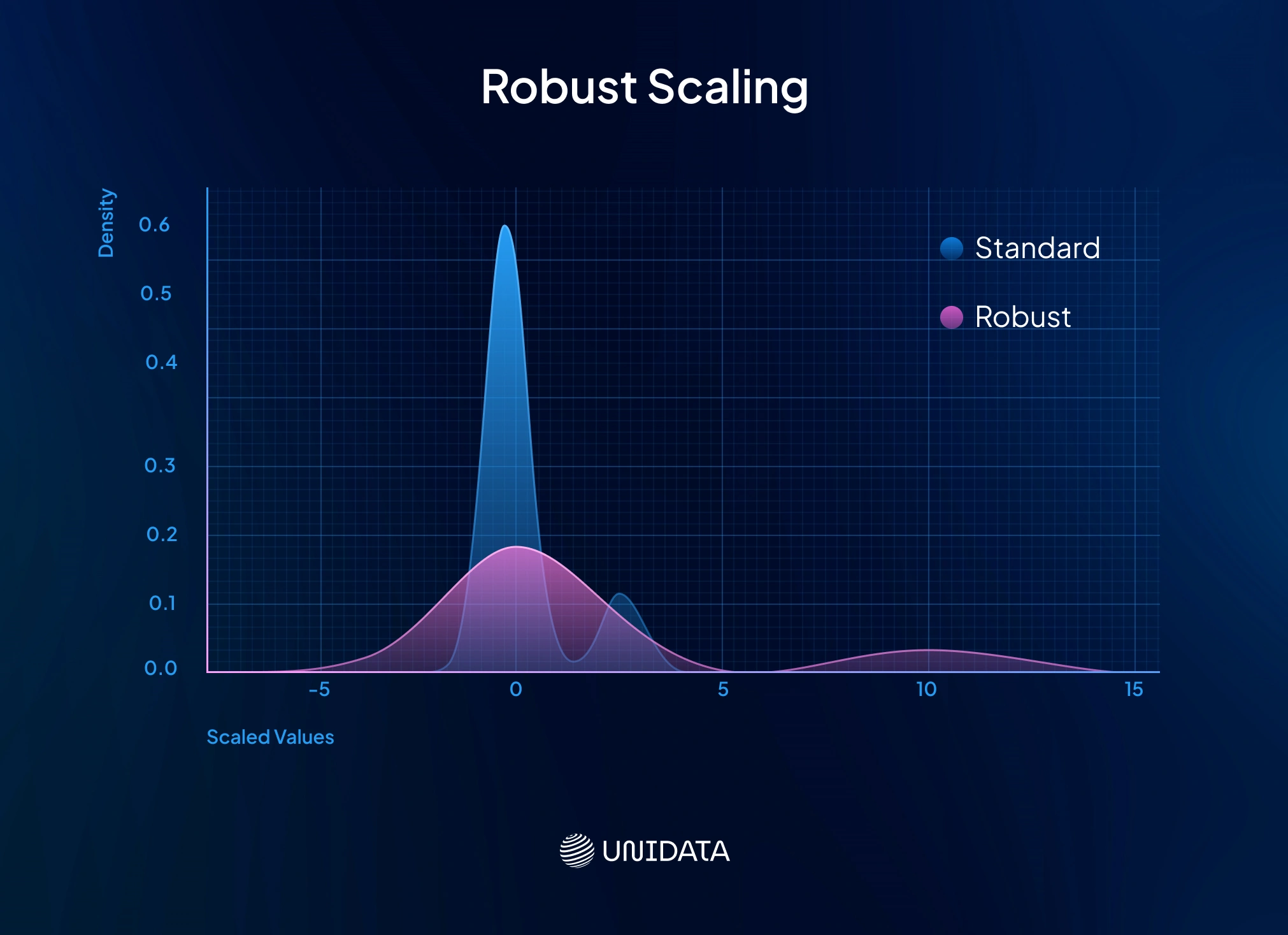
Robust scaling fights outliers head-on. Instead of chasing the mean and standard deviation, it locks onto the median and the interquartile range (IQR). Formula:
$$ x_{\text{scaled}} = \frac{x - \text{median}(x)}{\text{IQR}(x)} $$After scaling, the median is 0, and the middle 50 % of data points squeeze neatly into about [-0.5, 0.5].
Use cases
Perfect for skewed data with extreme outliers. Picture incomes: most between 30k–100k, a few in the millions. Standardization would blow up the millionaires’ z-scores and shrink the rest. Robust scaling locks onto the 30k–100k bulk, keeping features on a similar scale. It’s a good fit for long-tailed data like income, populations, or transaction counts.
Pitfalls
Outliers remain — they just don’t crush the middle. If data is close to a normal distribution, robust scaling may ignore useful variation in the tails. In that case, z score normalization works better.
Example
Housing lots: most are 0.1–0.5 acres, but a few farms hit 50. Min max scaling flattens normal homes near 0. Standardization throws farms 10σ out. With robust scaling, the median lot (0.2 acre) is 0, typical homes sit between -0.5 and 0.5, and farms stay far out — without skewing the rest.
Maximum Absolute Scaling (Max-Abs)
Max-Abs scaling is a twist on min max normalization. Each feature value is divided by the maximum absolute value in that feature. The result always falls in [-1, 1]. Unlike other methods, it doesn’t shift the mean — zeros stay zero.
$$ x_{\text{scaled}} = \frac{x}{\max(|x|)} $$Use cases
Best when data is sparse and full of zeros. In text classification or one-hot categorical features, most entries are 0. Standardization or min-max would distort those zeros. Max-Abs scaling leaves them untouched, while still putting all input features on a similar scale. That’s why it’s often the default in algorithms designed for sparse data.
Pitfalls
Outliers can break it. If one data point is extreme, the maximum absolute value shrinks everything else toward zero. It also doesn’t center the data, so any non-zero mean stays as bias. Sometimes it’s paired with mean subtraction when zeros don’t carry meaning.
Example
Picture a user-engagement vector: 100 actions, mostly zeros. Some users do 5 actions, some 10, one “super-user” does 50. With max-abs scaling, zeros stay 0, normal actions stay small, and the super-user caps at 1. Sparsity is preserved, and all the features contribute equally without warping the dataset.
Log Transformation
Log transformation isn’t linear scaling, but it reshapes feature values to shrink big gaps. By applying log (base 10 or natural), the high end compresses and the low end stretches. If zeros appear, a shift like log(x+1) is used.
Use cases
Great for features with a long right tail — income, population, sales, or anything that grows exponentially. The log pulls massive outliers back toward the pack and often makes the distribution closer to a Gaussian distribution. That helps algorithms, especially linear models, which assume more normal errors. For example, a raw gap of 1,000,000 vs. 10 shrinks from 100,000:1 down to 6:1 after log10.
Pitfalls
Logs fail on non-positive values. Negative numbers and zeros won’t work unless you add a constant. It also changes meaning: differences turn multiplicative, not additive. A jump from 100 to 200 is read as doubling, while 900 to 1000 becomes a small relative move. That’s often fine — just make sure it fits the business logic.
Example
Predicting housing prices with city population as a feature? Raw values from 1,000 to 8 million overwhelm the model. After log10, they shrink to ~3 to ~7. Now each order of magnitude — 10k, 100k, 1M — is evenly spaced. The feature becomes smoother, easier to handle, and still ready for extra scaling like min max normalization or z score normalization.
Comparison of Scaling Methods
Each method has pros and cons. Here’s a quick comparison of how they differ:
| Scaling Method | How It Works | Sensitive to Outliers? | When to Use |
|---|---|---|---|
| Min-Max Normalization (0–1) | Rescales feature to a fixed range (usually 0 to 1) based on min and max. Preserves relative ordering of data points. | High. A single outlier can compress all other values into a narrow range. | - Data with no significant outliers - Algorithms like neural nets that benefit from bounded inputs - When original min/max are meaningful (e.g. image pixels) |
| Standardization (Z-score) | Shifts data to mean = 0, std = 1 (unit variance). | Moderate. Outliers affect mean and std, but not as drastically as min-max. | - Common default for many machine learning algorithms (linear models, SVM, KNN, PCA) geeksforgeeks.org - When data is roughly symmetric or normal in shape - When using models that assume normality or benefit from equal variance |
| Robust Scaling | Uses median for centering (to 0) and IQR for scaling (to unit IQR). | Low. Ignores extreme values when scaling (they still exist but don’t influence the scale of central data). | - Data with outliers or heavy skew (long tails) - When median is a better “central” measure than mean (e.g. income, housing prices) |
| Max-Abs Scaling | Divides by the maximum absolute value, resulting in range [-1,1] (no centering). | High. An outlier max will scale down all other values a lot. | - Sparse features or one-hot encoded categorical features (preserves 0 as 0) - Data that is already centered at 0 or when zeroes need to remain zero |
| Log Transformation | Applies log (or log1p) to compress scale of high values (not linear scaling). | N/A (Not linear; reduces outlier magnitude by nature). | - Positive-valued data with exponential or skewed distribution - To meet linear model assumptions (making skewed data more normal). Often used in combination with one of the above scalers. |
Pitfalls and How to Choose the Right Scaler
Picking a scaler isn’t a checklist item — it’s closer to mixing sound in a studio. Each feature is an instrument, and the goal is balance. Too much bass, and you lose the melody. Too much treble, and it’s noise. Feature scaling works the same way: adjust wisely, or one feature will drown out the others.
Data leakage
One of the easiest mistakes is scaling the whole dataset at once. Do that, and your model “peeks” at the test data before training. Always fit scalers on the training data only, then apply them to the test dataset. Pipelines in libraries like scikit-learn handle this for you and should be your default.
Outliers and skew
Plain min max scaling or z score normalization can break if outliers are extreme. They stretch the scale and crush the rest of the values. For long-tailed data, reach for robust scaling, a log transformation, or clip extreme values first.
Zeros that matter
Sometimes zero has meaning — zero purchases really means none. Standardization shifts it to -μ/σ, which might blur the story. Max abs scaling or min max will keep zeros at zero, making them better for sparse vectors or binary categorical features. In fact, one-hot encodings (0/1) shouldn’t be scaled at all.
Different scalers for different features
You don’t have to pick one scaler for everything. Standardize most features, log-transform a skewed one, and leave binary columns untouched. The key is to keep this consistent with a pipeline so new input data gets the same treatment.
Model interpretability
Scaling changes the unit of coefficients in linear models. A weight on a standardized feature means “effect per 1 standard deviation change,” not per original unit. That’s often useful, but if stakeholders need raw units, invert the transform or explain clearly.
Inverse transforms
If you scale targets (say, predicting prices in log-dollars), remember to convert predictions back. Most libraries provide an inverse_transform for this.
Scaling in Practice: Python Examples with sklearn, NumPy
Scaling isn’t hard in Python — most of the heavy lifting is done for you. Here’s how it plays out in practice.
With scikit-learn
The sklearn.preprocessing module gives you ready-to-go scalers: StandardScaler, MinMaxScaler, RobustScaler, MaxAbsScaler. Fit them on training data only, then apply to the test dataset — this avoids leakage. Pipelines make this seamless.
from sklearn.preprocessing import StandardScaler, MinMaxScaler, RobustScaler

scaler = StandardScaler()
X_train_scaled = scaler.fit_transform(X_train)
X_test_scaled = scaler.transform(X_test)

minmax = MinMaxScaler()
X_train_mm = minmax.fit_transform(X_train)
X_test_mm = minmax.transform(X_test)
With NumPy
Scaling is just math. Use mean, std, min, max directly.
import numpy as np
X = X_train.values
X_train_std = (X - X.mean(axis=0)) / X.std(axis=0)
X_train_mm = (X - X.min(axis=0)) / (X.max(axis=0) - X.min(axis=0))
Remember to store parameters (mean, std, etc.) so you can scale new data the same way.
Quick demo
A column [1, 2, 3, 4, 100] shows how scalers react to an outlier:
- Min max scaling pushes 100 to 1.0, compressing small values near 0.
- Standardization gives mean 0, std 1; 100 ends ~+2.0.
- Robust scaling sets the median to 0, IQR to 1; 100 shoots to ~48, clearly flagged as an outlier.
The takeaway: different scaling techniques treat outliers very differently. Always sanity-check scaled values before feeding them into machine learning models.
Effect of Feature Scaling on Training vs Testing Data
Always fit the scaler on training data — then use it to transform validation and test dataset. Never refit on test. Doing so leaks information and makes your evaluation unreliable.
Why? Suppose test values run higher than train. If you include them when finding the minimum value or maximum value, your min max scaling shifts, and the model “learns” from data it shouldn’t have seen. Performance scores will look better than they really are.
The safe workflow:
- Fit scaler on training data.
- Transform train with saved parameters.
- Apply the same transform to validation and test.
Most libraries enforce this with fit_transform on train and transform on test. The same logic holds if you scale targets in regression — fit on train, transform test, and don’t forget to invert predictions back to original units.
Scaling is reversible. Keep your scaler object so new input data can be transformed the same way, and outputs returned in their original scale.
Feature Scaling and Gradient Descent Convergence
When features sit on different scales, gradient descent slows to a crawl. The loss surface stretches like a long ravine, forcing the algorithm to zigzag with tiny steps.
Scale the data, and the ravine becomes round. The optimizer moves straight to the minimum with fewer iterations and larger learning rates. Regularization also plays fair — penalties apply evenly across all the features instead of punishing those with bigger units.
If your model learns with gradient descent, scaling is a simple way to train faster and more reliably.
Scaling Numerical vs. Categorical Features
Not all features need the same treatment. Numerical features? Scale them with the right technique. Categorical features? Different story.
One-hot vectors (0/1) are already on a common scale. Don’t standardize them — it turns clean 0/1s into messy -0.3 and 2.9, which adds nothing and can even hurt models.
Ordinal encodings (e.g. education levels 0–3) aren’t true numbers. Scaling them won’t fix that. For tree-based models, raw codes are fine. For linear models, one-hot encoding is usually safer.
Binary flags (0/1) can stay as they are. They’re already simple and bounded. If you really want, apply max abs scaling, which keeps 0 as 0 and 1 as 1.
The rule of thumb: scale your numerical features carefully, but leave categorical features encoded and untouched. That way, you don’t introduce fake distances where none exist.
Conclusion
Feature scaling levels the playing field. It keeps one feature vector from dominating, speeds up gradient descent, and makes distance calculations fair in algorithms like k means clustering or support vector machines.
We covered the essentials: min max normalization, z score normalization, robust scaling, max abs scaling, and log transformation. Each has its role, from taming outliers to handling sparse input data. Real-world results prove it — scaling can turn a weak model into one that jumps from 35 % to 96 % accuracy.
The takeaway? Scaling isn’t polish. It’s core feature engineering in data science.