Imagine you’re navigating with a compass that is slightly off. Each step compounds the error, and before long you end up miles away from your intended destination. That’s what happens when machine‑learning (ML) models are trained and deployed without a clear sense of fairness. Small biases in data or algorithms can scale into systemic injustices, eroding trust and yielding poor decisions. Whether you build models or buy them, fairness isn’t just a technical footnote; it’s a moral and business imperative.
Fairness shapes the way ML systems impact people’s lives. When algorithms decide who gets a loan, a job interview, or access to healthcare, unfair models can reinforce historical discrimination. Several fairness metrics have been proposed to measure and mitigate such harms. This article decodes those metrics and explains how to use them in practice.
Why fairness matters in AI and ML
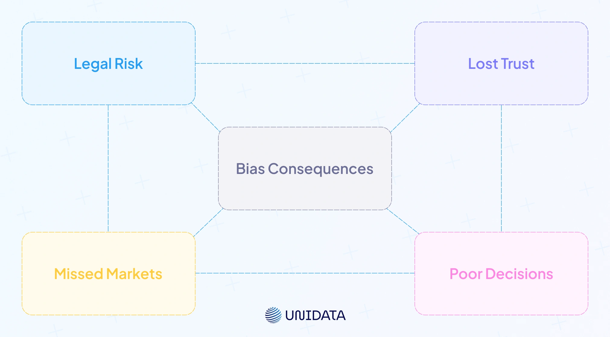
Fairness sits at the crossroads of ethics, law and business. Biased models can deny qualified applicants employment or credit opportunities, undermine public trust and expose organizations to legal risk. Beyond compliance, fairness fosters trust in AI: customers and employees are more likely to accept automated decisions when transparency and equity are at the core. In competitive markets, fairness also drives innovation by broadening the talent pool and avoiding costly reputational damage.
Defining fairness, bias and discrimination in algorithms
To talk about fairness metrics, we need clear definitions. Fairness refers to impartial and equitable treatment of individuals or groups. Bias means systematic error that favors certain outcomes. Biases are categorized into historical (legacy discrimination), representation (sample underrepresentation), measurement (poor proxies), aggregation (lumping groups together), evaluation (choosing the wrong metrics) and deployment bias. Discrimination occurs when an algorithm produces unequal outcomes based on protected attributes (race, gender, age) rather than merit.
Importantly, not all disparities are unfair. An ML model may legitimately allocate more resources to groups with higher needs. Fairness metrics therefore quantify whether disparities are justified or signal potential discrimination. Group fairness metrics evaluate outcomes across groups; individual fairness focuses on similar individuals receiving similar outcomes; causal fairness considers whether sensitive attributes causally influence predictions cran.r-project.org.
A taxonomy of fairness metrics
Fairness metrics can seem like a maze. Below is a structured taxonomy that maps the landscape.
Group fairness metrics
Group fairness evaluates whether groups defined by a sensitive attribute (e.g., gender, ethnicity) receive similar treatment. Key metrics include:
Demographic Parity (Independence) – A model satisfies demographic parity if the probability of a positive outcome does not depend on the sensitive attribute. Formally, independence requires:
$$ \frac{P(R=1 \mid A=a)}{1} = \frac{P(R=1 \mid A=b)}{1} $$In a hiring example, demographic parity means men and women are selected at the same rate ocw.mit.edu.
# Example: compute demographic parity difference in Fairlearn
from fairlearn.metrics import demographic_parity_difference
parity_diff = demographic_parity_difference(y_true, y_pred, sensitive_features)
This code computes the difference in selection rates between privileged and unprivileged groups. A value close to zero indicates parity.
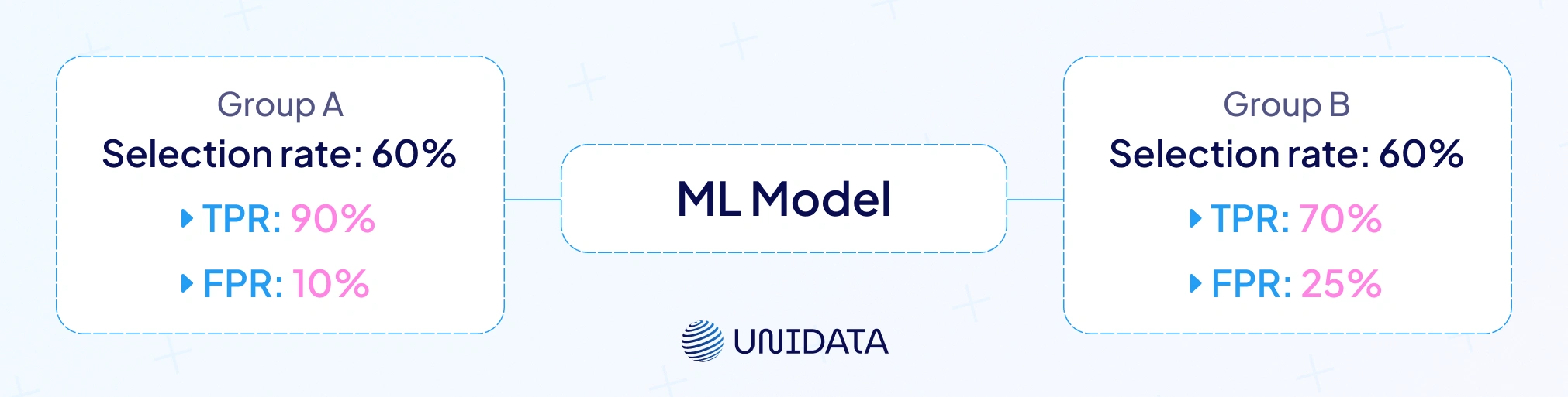
Equalized Odds (Separation) – Equalized odds require that the model’s true‑positive rate (TPR) and false‑positive rate (FPR) are equal across groups:
This metric ensures that the model performs equally well for each group ocw.mit.edu.
from fairlearn.metrics import equalized_odds_difference
eod_diff = equalized_odds_difference(y_true, y_pred, sensitive_features)
Equal Opportunity – A relaxed version of equalized odds requiring equal TPR across groups but allowing different FPR:
$$ \frac{P(R=1,\,Y=1 \mid A=a)}{P(Y=1 \mid A=a)} = \frac{P(R=1,\,Y=1 \mid A=b)}{P(Y=1 \mid A=b)} $$It is useful when false positives are less harmful than false negatives.
Predictive Parity (Sufficiency) – Also known as predictive parity or calibration, this metric mandates that the probability of a true outcome given a positive prediction is equal across groups:
$$ \frac{P(Y=1,\,R=1 \mid A=a)}{P(R=1 \mid A=a)} = \frac{P(Y=1,\,R=1 \mid A=b)}{P(R=1 \mid A=b)} $$It focuses on equal precision.
Statistical Parity Difference & Disparate Impact – Statistical parity difference measures the difference in positive outcome rates between unprivileged and privileged groups.
$$ \frac{P(R=1 \mid A=a)}{P(R=1 \mid A=b)} $$Disparate impact computes the ratio of these rates; values below 0.8 or above 1.25 suggest possible discrimination and may violate the four‑fifths rule.
Average Odds Difference – This metric averages the differences in FPR and TPR between groups. It aims to combine aspects of equalized odds into a single number.
PPV, FPR and NPV Parity – Positive predictive value (PPV) parity, false positive rate (FPR) parity and negative predictive value (NPV) parity require equal PPV, FPR and NPV across groups. Superwise’s fairness metrics article shows formulas for these metrics: for equalized odds, equal positive predictive value, equal false positive rate and equal negative predictive value. These metrics capture errors and successes in classification.
Recall Parity & False Positive Rate Parity – Recall (or true positive rate) parity ensures that recall is equal across groups; FPR parity demands equal false positive rates. Arize AI notes that fairness can be evaluated via recall parity and FPR parity to detect disparate error rates.
Theil Index & other disparity measures – Some frameworks compute the Theil index (inequality measure) or Gini coefficient to quantify unfairness. Although less common, they can help summarize disparities in continuous outcomes.
Individual fairness
Individual fairness posits that similar individuals should receive similar outcomes cran.r-project.org. Dwork et al.’s famous axiom expresses this concept. Measuring individual fairness requires a distance metric capturing similarity. Techniques include:
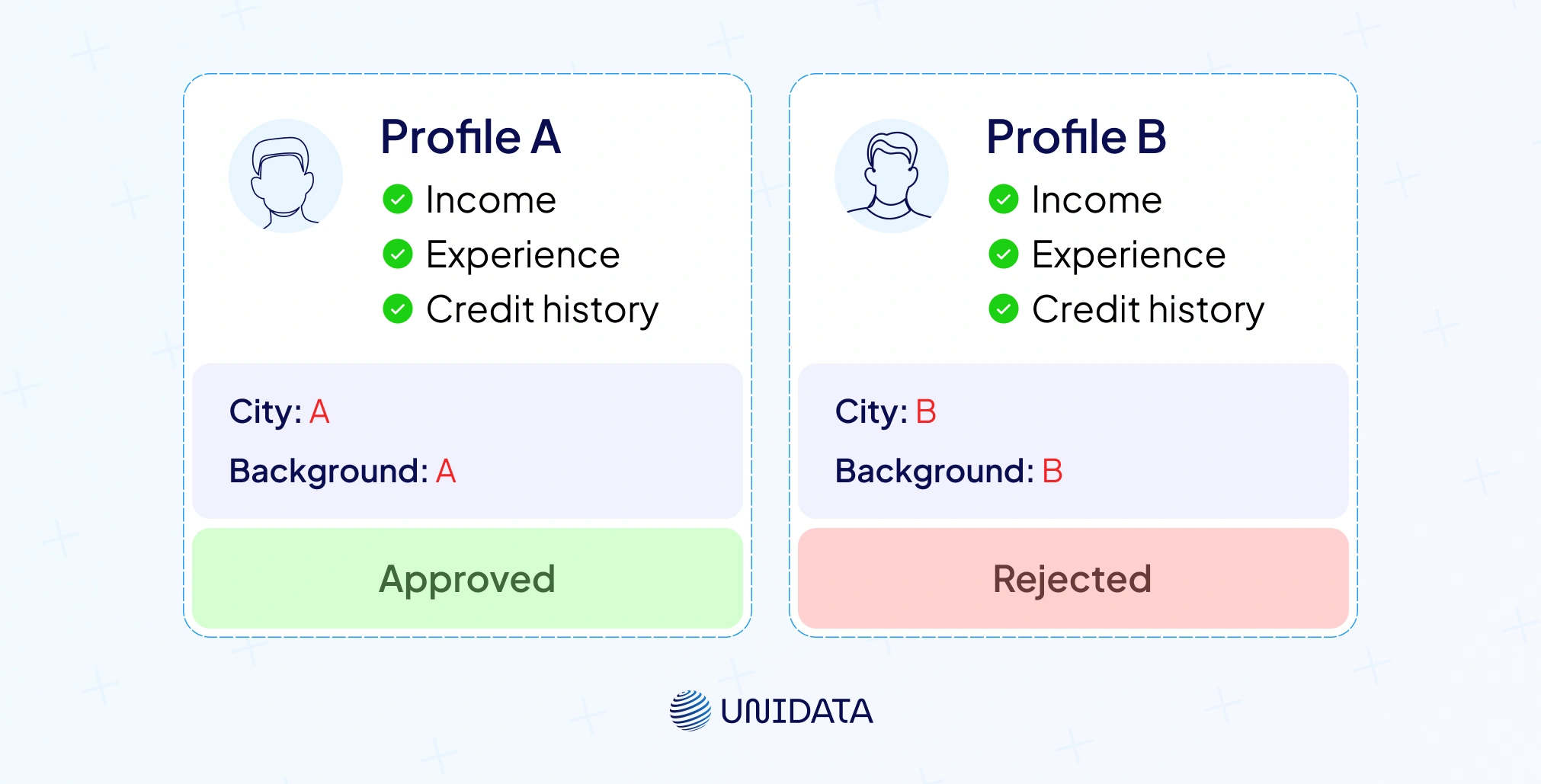
- Counterfactual fairness: evaluate whether a prediction would differ if the individual’s sensitive attribute changed, holding all else constant. If the outcome changes, the model may be unfair.
- Fairness through unawareness: simply removing sensitive attributes doesn’t guarantee fairness because proxies may exist in the data.
- Similarity metrics: define a distance function based on features such as credit history or performance. Individual fairness metrics assess whether prediction differences correlate with distances.
Causal fairness
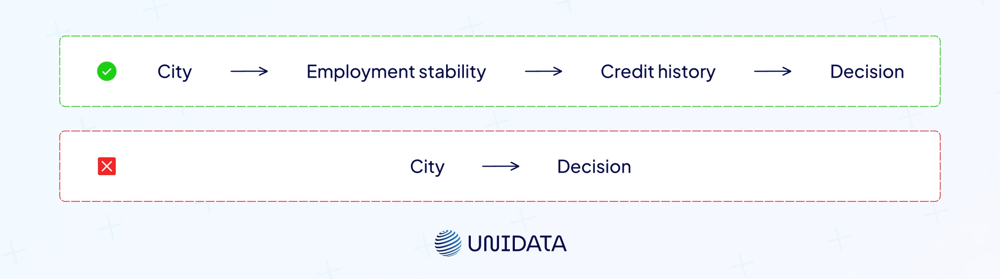
Causal fairness goes beyond observational statistics to ask whether sensitive attributes causally influence outcomes. If race influences a loan decision through a legitimate credit history channel, the causal effect may be justified. But if race influences outcomes directly, the model is unfair. Causal frameworks like counterfactual fairness use structural equation models to test these causal pathways.
Visual comparison of fairness metrics
A comparison table helps illustrate the strengths and limitations of each fairness metric. Keep in mind that no metric is universally “best”; each captures different notions of fairness.
| Metric | Definition | Pros | Cons |
|---|---|---|---|
| Demographic parity (independence) | Selection rate should be independent of sensitive attribute: $P(R=1 \mid A=a)=P(R=1 \mid A=b)$ | Simple to compute; addresses allocation harms | Can sacrifice accuracy; unfair to individuals if groups differ in qualification |
| Equalized odds (separation) | TPR and FPR equal across groups: $\frac{P(R=1,\,Y=1 \mid A=a)}{P(Y=1 \mid A=a)}=\frac{P(R=1,\,Y=1 \mid A=b)}{P(Y=1 \mid A=b)}$ | Balances error rates; good for quality of service | Difficult to satisfy with limited data; may reduce predictive accuracy |
| Equal opportunity | Equal TPR across groups: $\frac{P(R=1,\,Y=1 \mid A=a)}{P(Y=1 \mid A=a)}=\frac{P(R=1,\,Y=1 \mid A=b)}{P(Y=1 \mid A=b)}$ | Ensures qualified individuals have equal chance; easier than equalized odds | Allows different FPRs; may still harm one group |
| Predictive parity (sufficiency) | Equal precision: $\frac{P(Y=1,\,R=1 \mid A=a)}{P(R=1 \mid A=a)}=\frac{P(Y=1,\,R=1 \mid A=b)}{P(R=1 \mid A=b)}$ | Aligns with accuracy; ensures predictions are equally reliable | Can conflict with equalized odds and demographic parity |
| Statistical parity difference | Difference in positive outcome rates: $P(R=1 \mid A=a) - P(R=1 \mid A=b)$ | Easy to interpret; aligns with four‑fifths rule | Ignores errors; may hide disparate mistakes |
| Disparate impact (ratio) | Ratio of positive outcome rates; fair if 0.8–1.25 | Used in legal contexts; simple threshold | Doesn’t capture error rates or individual fairness |
| Average odds difference | Average of TPR and FPR differences | Single measure summarizing equalized odds | May hide unequal tradeoffs between TPR and FPR |
| PPV/FPR/NPV/Recall parity | Equal PPV, FPR, NPV or recall across groups | Focus on specific error types; domain‑specific | Many metrics to track; may conflict with other fairness goals |
How fairness metrics fit into model development
Fairness isn’t an afterthought; it’s an integral part of the ML lifecycle. Below is a step‑by‑step process that integrates fairness metrics at each stage:
Data collection and labeling
Biases often originate from data. Historical discrimination, measurement errors and underrepresentation can skew training data. Ethical data sourcing and diverse representation are critical. Consider fairness-aware data labeling pipelines that actively monitor representation.
Exploratory analysis
Before training, evaluate group statistics. Compute the base rates of positive outcomes across sensitive groups and look for disparities. Use statistical parity difference and disparate impact to identify imbalances.
Model training with fairness constraints
Incorporate fairness metrics into the objective function. Fairlearn, for example, allows you to specify a fairness constraint (e.g., demographic parity or equalized odds) and learns a model that balances accuracy and fairness. An in‑processing approach can add a regularization term penalizing unfairness.
 # Fairlearn: train a classifier with an equalized odds constraint
from fairlearn.reductions import ExponentiatedGradient, EqualizedOdds
from sklearn.linear_model import LogisticRegression
constraint = EqualizedOdds()
clf = ExponentiatedGradient(LogisticRegression(), constraint)
clf.fit(X_train, y_train, sensitive_features=sensitive_attr)
y_pred = clf.predict(X_test)
Model evaluation
Evaluate both accuracy metrics (precision, recall, F1) and fairness metrics. Fairness metrics often trade off against accuracy, so choose the right balance for your domain.
Adversarial debiasing and learning fair representations
Bias mitigation can occur at different stages:
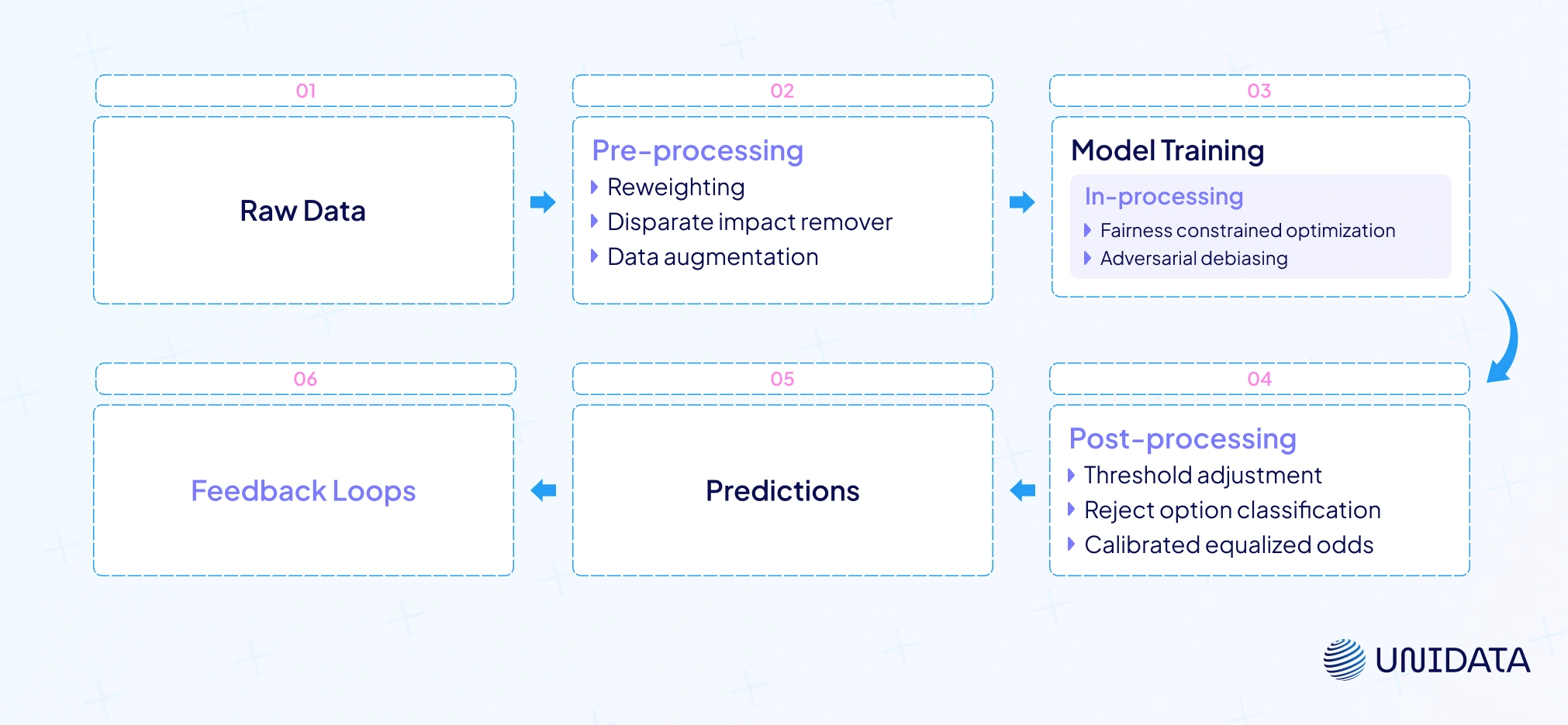
Pre‑processing techniques
These methods transform the dataset before training to reduce correlation between sensitive attributes and outcomes:
- Reweighting: assign weights to samples so that each group contributes equally to the loss function.
- Disparate impact remover: edit feature values to mitigate correlation with sensitive attributes.
- Data augmentation: oversample underrepresented groups or generate synthetic data.
In‑processing techniques
These techniques modify the training algorithm to include fairness constraints or adversarial objectives:
- Fairness constrained optimization: incorporate constraints like demographic parity into the loss function.
- Adversarial debiasing: train a predictor and an adversary simultaneously. The predictor minimizes prediction error while the adversary tries to predict the sensitive attribute from the predictor’s output. The predictor learns representations that obfuscate sensitive attributes, reducing bias. Adversarial debiasing and fair representation learning are effective in de‑correlating model outputs from sensitive features.
Post‑processing techniques
After training, you can adjust the model’s predictions without modifying the model itself. For example:
- Threshold adjustment: set different decision thresholds for different groups to satisfy fairness constraints like equalized odds.
- Reject option classification: flip predictions near the decision boundary for unprivileged groups to improve fairness.
- Calibrated equalized odds: adjust the predicted probabilities to equalize odds while maintaining calibration.
Feedback loops and model drift
Models don’t operate in a vacuum. Their predictions influence the environment, which in turn affects future data — a feedback loop. For instance, a predictive policing model that sends more patrols to certain neighborhoods may record more incidents there, reinforcing the model’s belief that those areas are high risk. Over time, this drift can amplify bias. Continuous monitoring of fairness metrics helps detect and mitigate such drifts. Retraining on updated, balanced data and using fairness constraints in production can reduce feedback effects.
Navigating trade‑offs: accuracy vs fairness and more
Fairness rarely comes for free. Improving one fairness metric often worsens another or reduces accuracy. For example, achieving demographic parity may require lowering the threshold for unprivileged groups, increasing false positives. Equalized odds may sacrifice calibration or predictive parity. Organizations must evaluate the trade‑off between fairness and performance, possibly accepting some performance loss to achieve fairness.
There is also tension between group fairness and individual fairness. Demographic parity treats groups equally, but individuals within groups may differ widely; equalized odds ensures equal error rates but may still treat similar individuals differently if they belong to different groups. In practice, you must prioritize fairness notions aligned with your mission, legal obligations and stakeholder expectations.
Fairness decision tree
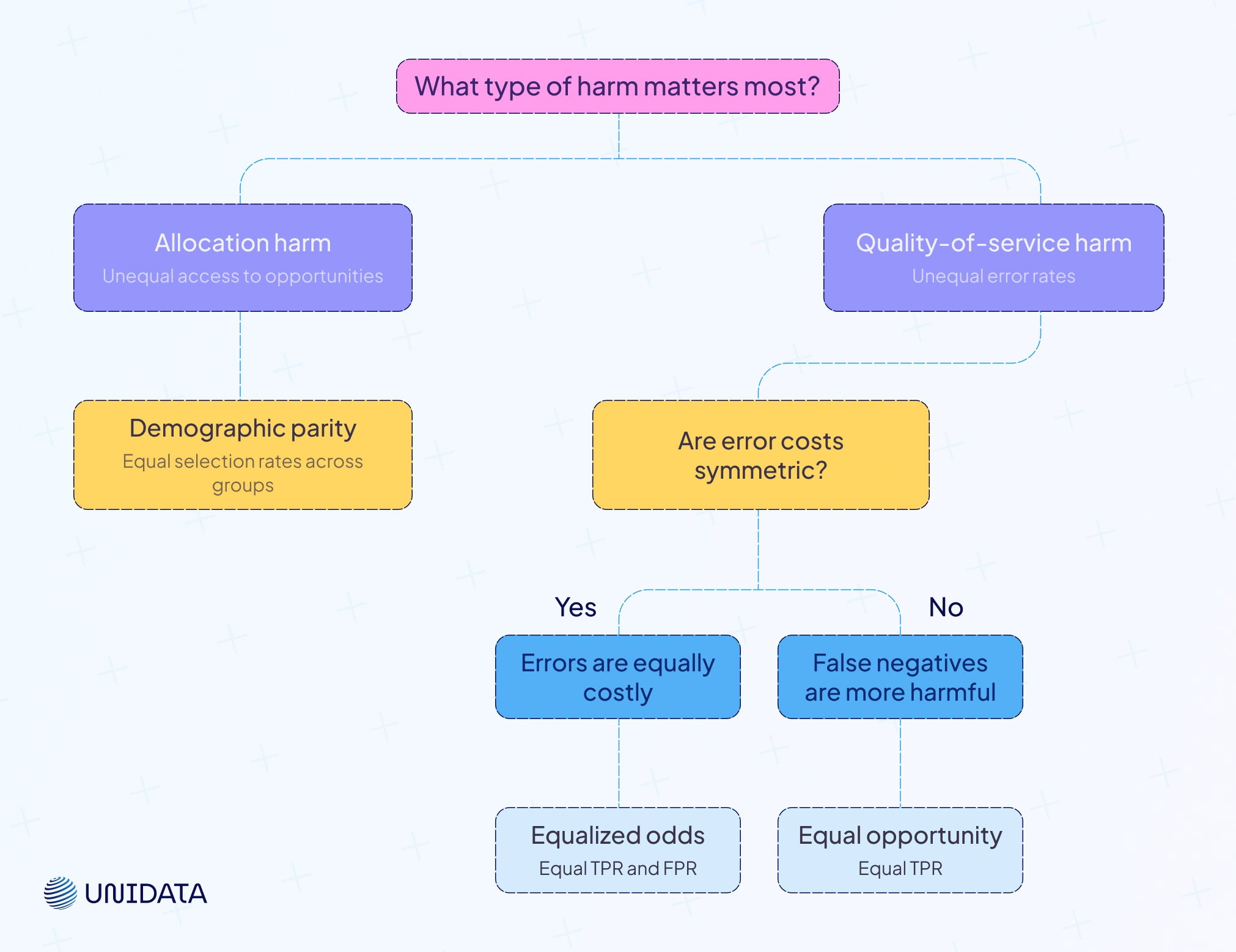
One way to manage trade‑offs is to use a fairness decision tree: identify the type of harm you want to mitigate (allocation vs quality of service), decide whether misclassification costs are symmetric or asymmetric, and choose metrics accordingly. For example, in hiring decisions, failing to hire a qualified candidate may be more harmful than hiring an unqualified one, so equal opportunity (equal TPR) may be prioritized.
Regulatory and ethical context
Fairness metrics interface with law and ethics. The four‑fifths rule from the U.S. EEOC suggests that selection rates for unprivileged groups should not be less than 80 % of the rate for privileged groups. However, the Fairlearn documentation warns that this rule is often misapplied and may conflate fairness with legality fairlearn.org. Similarly, demographic parity might meet the four‑fifths rule but still be unfair if groups differ in qualifications.
The emerging EU AI Act proposes risk‑based classifications requiring providers of high‑risk AI systems to conduct impact assessments, ensure transparency and include human oversight. Organizations may need to demonstrate that their models satisfy specific fairness metrics and provide explanations. Transparency and explainability are thus essential companions to fairness. Tools like Shapley values, counterfactual explanations and fairness dashboards help stakeholders understand why a model made a decision and how fairness metrics were computed.
Case studies: fairness in action
Credit scoring
Credit decisions have historically disadvantaged minorities. Suppose a lender trains a model to predict loan default. An audit reveals that the approval rate for minority applicants is 60 % of the majority’s rate, triggering the four‑fifths rule. By applying a reweighting technique and adding equalized odds constraints during training, the lender reduces the disparity and achieves equal TPR and FPR across groups. However, the model’s overall default prediction accuracy drops by 2 %. Stakeholders decide this trade‑off is acceptable because it improves fairness and reduces legal risk.
Criminal justice and risk assessment
The COMPAS recidivism risk score has been criticized for racial bias. Researchers found that while the system achieved similar predictive parity (PPV) across races, it failed equalized odds: Black defendants had higher false‑positive rates and lower true‑positive rates compared to white defendants. This illustrates the conflict between predictive parity and equalized odds. A possible remedy is to recalibrate the model under equalized odds, ensuring that error rates are similar across races even if precision varies.
Business ROI and trust benefits of fairness compliance
Beyond ethics and regulation, fairness makes business sense. Customers are increasingly aware of algorithmic bias; brands seen as discriminatory face boycotts and lawsuits. Fairness compliance reduces legal liability, protects reputation and unlocks broader markets. Fairness also supports trustworthy AI — a cornerstone for adopting AI in sensitive domains. Investors, regulators and consumers all scrutinize fairness metrics as signals of responsible AI. Achieving fairness can thus be a competitive advantage.
Conclusion
Fairness metrics are more than numbers. They embody our values and help ensure that machine‑learning systems serve everyone equitably. There is no one‑size‑fits‑all fairness metric; each captures different ethical priorities and involves trade‑offs. By understanding demographic parity, equalized odds, predictive parity and other metrics; integrating fairness into data collection, model training and deployment, you can build models that are both accurate and fair. Continue monitoring fairness, engage stakeholders and stay abreast of evolving regulations.