Ever tried teaching a friend a secret code? Suppose you decide to replace the word “apple” with the number 1, “banana” with 2, and “cherry” with 3. It works — each fruit gets a number. But what if your friend thinks 3 means better than 1 because it’s higher? Alternatively, you could send a separate signal for each fruit — like turning on a unique light for apple, banana, or cherry. Both methods convey the message in numbers, but one might accidentally imply a ranking that isn’t there.
This little dilemma is exactly what we face in machine learning when converting categories to numbers. In this article, we’ll unravel the differences between one-hot encoding and label encoding (our two “secret code” strategies) and then venture beyond to more advanced techniques. By the end, you’ll know how to translate categorical data for your models like a pro — without losing meaning in translation.
What Are Categorical Variables (and Why Encoding Matters)?

Categorical variables are labels, not amounts. They are classic categorical data like color, country, product ID, disease type, or credit rating. Think of encoding as a passport. Without it, your data can’t enter models.
They come in two flavors:
- Nominal data: no inherent order. Example: red, blue, green.
- Ordinal data: a natural order exists, like low < medium < high. The steps, however, aren’t equal.
Most machine learning algorithms expect a numerical format, not text. That’s why we encode categorical variables into numbers the model can learn from.
The encoding method changes how models read your data. Label encoding assigns an integer value to each class. It works well for ordinal data. But for pure nominal, it’s risky — models may infer rank from the numbers. One hot encoding avoids this by creating new binary columns for each category. The trade-off? It can increase dimensionality quickly when there are many unique categories (scikit-learn).
One-Hot Encoding Explained
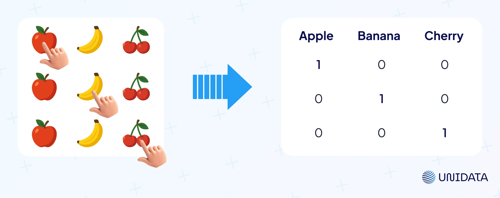
Think “one switch per value.” One hot encoding turns a category into new binary columns. For example, if we have a feature Color with values {Red, Green, Blue}, one-hot encoding will create three new columns: Color_red, Color_green, Color_blue. A red item becomes Color_red=1, Color_green=0, Color_blue=0; a blue item becomes 0,0,1, and so on. No fake ranking. Just on/off.
That’s why it fits nominal data. Categories are distinct. No ordinal relationship implied. Models see a clean numerical format without “Blue > Green” mistakes (scikit-learn).
Let’s see one-hot encoding in action with a simple example and Python code. Suppose we have a dataset of fruits with a Type column:
import pandas as pd

# Sample data
df = pd.DataFrame({'Fruit': ['Apple', 'Banana', 'Cherry', 'Apple', 'Cherry']})
print("Original DataFrame:")
print(df)

# One-hot encode the 'Fruit' column
one_hot = pd.get_dummies(df['Fruit'])
print("\nOne-hot encoded columns:")
print(one_hot)
Running this would produce something like:
Original DataFrame:
    Fruit
0   Apple
1  Banana
2  Cherry
3   Apple
4  Cherry

One-hot encoded columns:
   Apple  Banana  Cherry
0      1       0       0
1      0       1       0
2      0       0       1
3      1       0       0
4      0       0       1
Each fruit is now represented by a vector of 0s and 1s indicating its category. The model can now use these binary features directly.
Tooling is easy: pandas.get_dummies, scikit-learn pipelines, and most machine learning algorithms accept the transformed data. In NLP, bag-of-words is one giant version of this idea. Neural nets and linear models love the clarity.
Pros
Interpretable. Each category has its own weight. Great when unique categories are few. Works nicely with logistic/linear regression and even decision trees/random forests.
Cons
It can increase dimensionality fast. 100 unique values → 100 new columns. You get a huge feature space full of zeros. Training slows. Memory spikes. Sparse features can hurt some pipelines (IBM: categorical data).
Where it shines: gender, blood type, payment method — small sets. Where it stumbles: thousands of product IDs or diagnosis codes. For those, consider alternatives before you explode the matrix.
Label Encoding (Ordinal Encoding) Explained
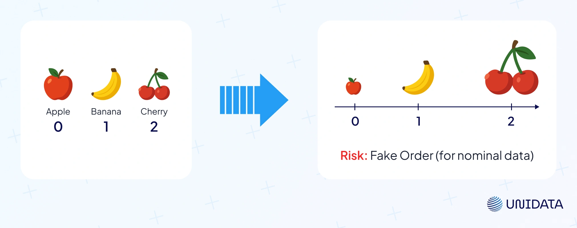
Label encoding takes the simple route: replace each category with an integer value.
Example: {'Apple': 0, 'Banana': 1, 'Cherry': 2}. Same idea as giving apple=1, banana=2, cherry=3. If categories have an ordinal relationship, we respect that order. If not, the numbering is arbitrary (often alphabetical or by appearance).
Here’s a quick example using pandas to label encode:
# Continuing from the previous DataFrame df
df['Fruit_label'] = df['Fruit'].astype('category').cat.codes
print("Label encoded DataFrame:")
print(df)
This might output:
Label encoded DataFrame:
    Fruit  Fruit_label
0   Apple            0
1  Banana            1
2  Cherry            2
3   Apple            0
4  Cherry            2
Now the Fruit column is encoded as 0, 1, 2. You could also use scikit-learn’s LabelEncoder for a single column, or OrdinalEncoder when handling multiple categorical variables.
Pros
It’s compact and memory-friendly. No new columns, just one. Perfect for ordinal data like T-shirt sizes (S < M < L < XL) or credit ratings. Numeric models can learn increasing or decreasing effects — e.g., XL (4) > S (1). Some tree based models (like decision trees or random forests) also work fine with label codes, since they can split the range of codes into groups.
Cons
For nominal categories, it may imply a false order. A model might read Cherry=2 > Banana=1 > Apple=0 as a real hierarchy, which makes no sense (Statology). Linear regression, SVMs, or KNN can misinterpret those numbers as magnitudes. Another drawback: one column may not capture complex category effects, so linear models lose flexibility compared to one-hot encoding.
When to use it
Use label encoding when natural order matters: survey ratings, credit scores, education levels. It can also be a quick fix in tree-based algorithms with high-cardinality features like ZIP codes or product IDs. But beware: arbitrary numbering can cause odd splits. That’s why tools like CatBoost use smarter internal encodings to avoid those pitfalls.
One-Hot vs. Label Encoding: How to Choose?
Now that we’ve covered the basics, the big question is simple: which encoding method when? It depends on your categorical variables and the machine learning algorithms you use.
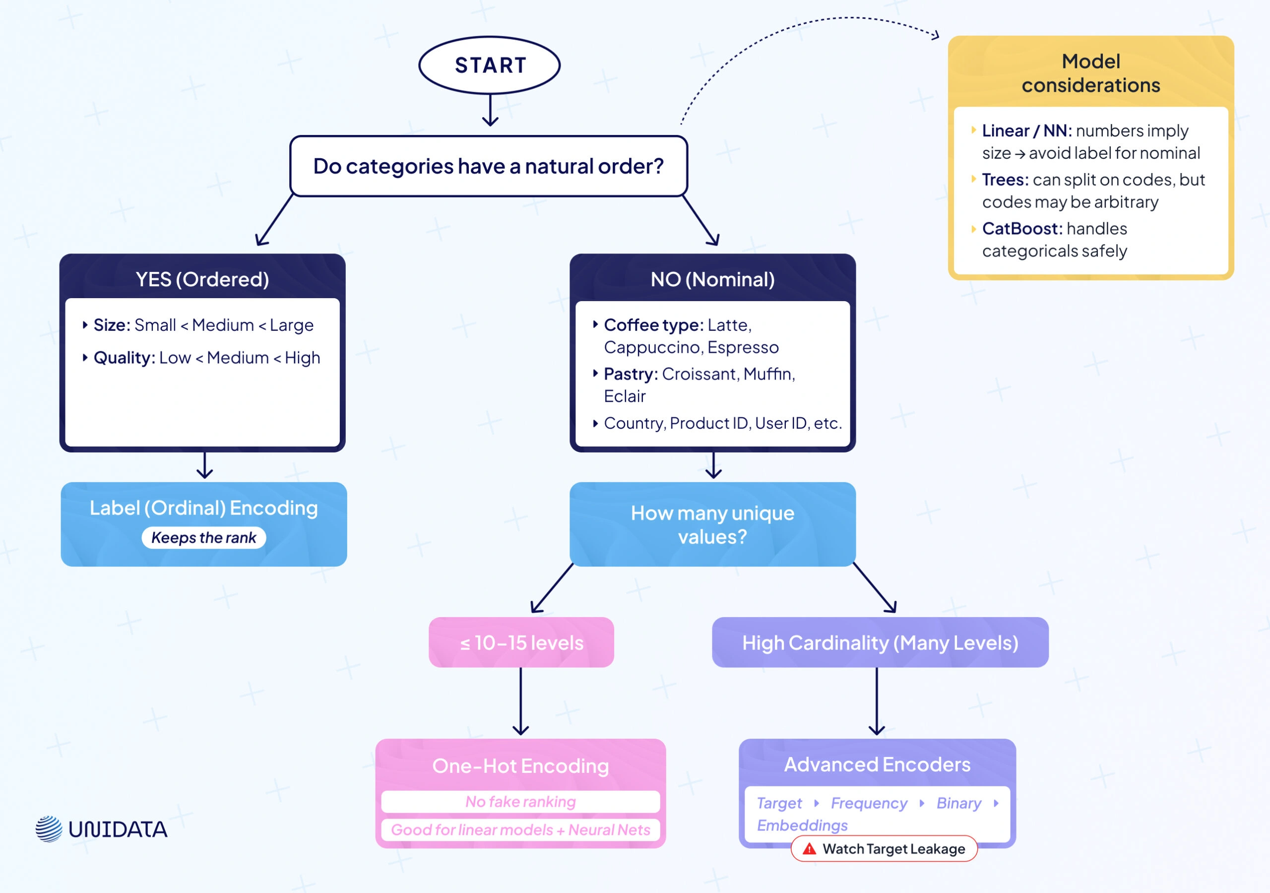
Use One-Hot Encoding for Nominal Data
No natural order? Go one hot encoding. You get new binary columns and no fake ranking. Great for colors, product IDs, user IDs, countries — when unique values are manageable. Safer for linear models and neural nets that read magnitudes.
Use Label (Ordinal) Encoding for Ordered Data
Have a natural order? Choose label encoding. Keep the ordinal relationship (low < medium < high). One-hot would treat levels as unrelated and throw away rank.
Consider Cardinality
A handful of levels (≈ ≤ 10—15) plays well with one-hot. Dozens or hundreds of unique categories? One-hot will increase dimensionality and bloat the feature space. Prefer label encoding or advanced methods when levels explode.
Model Considerations
- Linear/logistic regression and neural networks treat numbers as size. Label-encoding nominal categories can inject a fake order. One-hot is safer here.
- Tree-based models (decision trees, random forests, boosting) can split on label codes and group categories. Still, splits are one-dimensional; numeric codes aren’t always meaningful. Libraries like CatBoost handle categorical data with target-stat tricks to avoid pitfalls.
| Encoding Method | Best For | Advantages | Disadvantages |
|---|---|---|---|
| One-Hot Encoding | Nominal categorical variables with relatively few unique values (e.g. colors, gender, blood type). | - No false ordinal relationships imposed (each category is independent).- Widely supported and produces human-interpretable features (dummy vars). | - Expands feature dimension significantly if many categories (e.g. 100 unique values → 100 new columns).- Can be memory-inefficient and lead to sparse data, which some models struggle with. |
| Label Encoding (Ordinal Encoding) | Ordinal categories where order matters (e.g. low/medium/high, education level) or when using tree-based models with high-cardinality nominal data as a workaround. | - Preserves natural order of categories when one exists (model can learn increasing/decreasing effects).- Very compact representation (one column, no expansion), making it computationally efficient. | - Implies an arbitrary ranking for nominal categories, which can mislead many models (e.g. “Cherry=3” > “Apple=1” even if no real rank).- For nominal data, it may reduce model flexibility (linear model assumes a single slope across the coded values). |
Beyond One-Hot and Label: Advanced Encoding Techniques
Real datasets are messy. In finance, retail, and healthcare, categorical variables can have thousands of unique categories. One hot encoding blows up the feature space. Label encoding can add a fake ordinal relationship. We need more options.
Here are four solid encoding methods to use when basics fail: target encoding, frequency encoding, binary encoding, and learned embeddings. They keep useful signal, control size, and play nicely with different machine learning algorithms (scikit-learn).
Target Encoding (Mean Encoding)
What it is
A supervised encoder. Replace each category with a summary of the target for that category — mean for regression, class probability for classification. For example, suppose you’re predicting house prices and one of your categorical features is “Neighborhood.” With target encoding, you would calculate the average house price for each neighborhood in your training data, and use those averages as the encoded values for that feature. A fancy neighborhood gets a high number, an average neighborhood a moderate number, etc.
In effect, target encoding answers: “based on training data, how predictive is this category of the outcome?” It can be very powerful — you’re giving the model a head start by providing a distilled effect of each category. In fact, when there is a strong relationship between the category and the target, this can significantly boost model performance.
Let’s illustrate with code
We’ll do a tiny retail example: predict Sales and encode Store_ID with its mean Sales.
import pandas as pd

# Sample data
df_sales = pd.DataFrame({
    'Store_ID': ['A', 'B', 'C', 'A', 'B', 'C'],
    'Sales': [100, 200, 300, 150, 250, 350]
})
print("Original Data:")
print(df_sales)

# Compute mean Sales per Store_ID (target encoding mapping)
target_mean = df_sales.groupby('Store_ID')['Sales'].mean()
print("\nMean Sales per Store (for encoding):")
print(target_mean)

# Map the mean to each Store_ID
df_sales['Store_encoded'] = df_sales['Store_ID'].map(target_mean)
print("\nData with Target-Encoded Store_ID:")
print(df_sales)
Output might be:
Original Data:
  Store_ID  Sales
0        A    100
1        B    200
2        C    300
3        A    150
4        B    250
5        C    350

Mean Sales per Store (for encoding):
Store_ID
A    125.0
B    225.0
C    325.0
Name: Sales, dtype: float64

Data with Target-Encoded Store_ID:
  Store_ID  Sales  Store_encoded
0        A    100          125.0
1        B    200          225.0
2        C    300          325.0
3        A    150          125.0
4        B    250          225.0
5        C    350          325.0
We replaced Store_ID with the average sales of that store in the dataset. Store A is encoded as 125, B as 225, C as 325 (their average sales). If we feed this to a model, the feature now directly carries information about likely sales. This technique shines in high-cardinality situations — e.g., encoding user IDs by their average purchase amount, encoding zip codes by average income or default rate, etc.
Pros
Huge drop in dimensionality. Clear numerical format with useful signal. Often boosts machine learning models on high-cardinality features.
Cons
Risk of target leakage. Never compute means on the full dataset. Use cross-fitting and smoothing (blend category mean with the global mean) to avoid overfitting. Less interpretable than one-hot.
When to use
High-cardinality features with real signal: occupations → claim rate, campaigns → conversion rate, stores → average sales. Popular in practice; some libraries do a version of this internally (CatBoost’s target-style stats: docs).
Frequency Encoding (Count Encoding)
What it is
Replace each category with how often it appears. You map a label to its count (or frequency in the dataset). Essentially, you’re encoding each category by its popularity. For example, if “Apple” appears 50 times in your data and “Cherry” appears 5 times, a frequency encoding might map Apple→50, Cherry→5. Sometimes this is scaled as a frequency (proportion of dataset) instead of raw count, but the idea is the same.
It answers: “how common is this category?” Models can use that signal, especially trees. It’s handy when you face high-cardinality categorical variables and want to avoid a huge feature space (CountEncoder — scikit-learn-contrib/category_encoders).
Let’s illustrate with code
We take Fruit → map to counts (Apple=50, Banana=20, Cherry=5).
df_freq = pd.DataFrame({'Fruit': ['Apple','Banana','Cherry','Apple','Banana','Apple']})
print("Original Data:")
print(df_freq)

# Frequency encode 'Fruit'
freq = df_freq['Fruit'].value_counts()
df_freq['Fruit_freq'] = df_freq['Fruit'].map(freq)
print("\nFrequency Encoded Data:")
print(df_freq)
Output:
Original Data:
    Fruit
0   Apple
1  Banana
2  Cherry
3   Apple
4  Banana
5   Apple

Frequency Encoded Data:
    Fruit  Fruit_freq
0   Apple           3
1  Banana           2
2  Cherry           1
3   Apple           3
4  Banana           2
5   Apple           3
Apple appears 3 times, Banana 2, Cherry 1, so we encoded those frequencies. A model might infer, for instance, that a fruit with frequency 1 (Cherry) could behave differently than a fruit with frequency 3 (Apple) if frequency correlates with something — for example, maybe rare fruits are more expensive, etc.
Pros
One column. Fast. No target leakage. Plays well with tree based models.
Cons
Same count ≠ same effect. Different categories can share the same number. No direct target signal.
When to use
Lots of unique values (IDs, ZIPs). You want compact features, not 1,000 dummies.
Binary Encoding
Binary encoding mixes the ideas of label encoding and one hot encoding. First, every category gets a number. Then that number is written in binary form. Each binary digit becomes its own column with 0s and 1s.
For example, suppose you have 8 categories labeled 0 through 7. In binary, 0 = 000, 1 = 001, ..., 7 = 111 (using 3 bits to cover 0-7). Binary encoding would create 3 new features (bit1, bit2, bit4 for example) instead of 8 one-hot features. Category 3 (which is binary 011) would be encoded as bit1=1, bit2=1, bit4=0. Category 7 (111) becomes 1,1,1; category 0 (000) becomes 0,0,0, etc.
Let’s do a quick binary encoding by hand to illustrate:
import numpy as np

df_bin = pd.DataFrame({'Category': ['A','B','C','D','E']})
# Label encode first
df_bin['Cat_code'] = df_bin['Category'].astype('category').cat.codes  # A=0, B=1, C=2, D=3, E=4
# Determine number of bits needed
n_categories = df_bin['Cat_code'].nunique()
n_bits = int(np.ceil(np.log2(n_categories)))
print(f"Using {n_bits} bits for {n_categories} categories.")
# Convert each code to binary string with padding
df_bin['Cat_binary'] = df_bin['Cat_code'].apply(lambda x: format(x, f'0{n_bits}b'))
# Split the binary string into separate bit columns
for i in range(n_bits):
    df_bin[f'Bit_{i}'] = df_bin['Cat_binary'].str[i].astype(int)

print(df_bin[['Category','Cat_code','Cat_binary','Bit_0','Bit_1','Bit_2']])
Assuming categories A-E got codes 0-4, this might output:
Using 3 bits for 5 categories.
  Category  Cat_code Cat_binary  Bit_0  Bit_1  Bit_2
0        A         0        000      0      0      0
1        B         1        001      0      0      1
2        C         2        010      0      1      0
3        D         3        011      0      1      1
4        E         4        100      1      0      0
We needed 3 bits for 5 values (since 2 bits can only represent 4 values). The bits columns (Bit_0 is the most significant bit here, Bit_2 the least in my naming) show the binary representation.
Pros
Huge size cut vs one hot encoding. Good for high-cardinality categorical data. Often friendly to decision trees/random forests.
Cons
Bits are not interpretable. Categories share bits, so models may need multiple splits to separate them.
When to use
Many unique categories; you need compact features and can trade some clarity for scale.
Learned Embeddings
The most advanced approach we’ll cover is learned embeddings — essentially letting the model learn its own encoding for the categories. This is typically done in the context of neural networks. Instead of manually encoding a categorical variable into fixed columns, you represent each category as an embedding vector (a small dense vector of numbers) and allow the neural network to optimize those vectors during training.
Why this is powerful
It combines the strengths of one-hot (no pre-imposed hierarchy) with automatic grouping like target encoding, but in a fully data-driven way. A properly learned embedding can capture subtle relationships between categories — for example, it might learn that two products are similar because they lead to similar purchasing patterns.
Let’s illustrate with code
Using TensorFlow/Keras to create an embedding for a feature:
import tensorflow as tf

# Suppose we have a feature 'City_ID' with 100 unique cities
city_count = 100
embed_dim = 5  # we choose to represent each city by a 5-dimensional vector

# Define an embedding layer for City
city_input = tf.keras.Input(shape=(1,), dtype='int32', name='city_input')
city_embedding = tf.keras.layers.Embedding(input_dim=city_count, output_dim=embed_dim, name='city_embed')(city_input)
city_embed_flat = tf.keras.layers.Flatten()(city_embedding)

# ... define other parts of the model, then concatenate and add output layer ...
# For simplicity, assume we directly output from the embedding:
output = tf.keras.layers.Dense(1, activation='linear')(city_embed_flat)
model = tf.keras.Model(inputs=city_input, outputs=output)
model.compile(optimizer='adam', loss='mse')
model.summary()
This sets up a model where each city is represented by a 5-length vector that will be learned. Initially, the city_embed weights are random. During training (say, predicting house prices from city), the network will adjust these vectors such that cities with higher prices get embeddings that help predict higher output, etc.
Pros
Captures similarity. Scales to thousands of categories. Often lifts machine learning models when data is rich.
Cons
Needs a neural network and enough data. Harder to interpret than one hot. Handle unseen categories with care.
When to use
You have many categories, plenty of data, and you want maximum accuracy (recsys, pricing, risk).
Comparison: Which Encoding Method to Use When?
We’ve covered a lot of ground. It’s helpful now to summarize and compare these encoding methods across a few dimensions: their ideal use cases, pros/cons, and scalability. The table below provides a side-by-side comparison:
| Encoding Method | Best For | Advantages | Drawbacks |
|---|---|---|---|
| One-Hot | Nominal data, low cardinality | Clear, no fake order, works in linear/NN | Too many columns if categories >15 |
| Label (Ordinal) | Ordered categories | Compact, keeps rank | Misleads if data is nominal |
| Target (Mean) | High-cardinality with signal | Small, adds predictive power | Risk of leakage, needs cross-val |
| Frequency (Count) | High-cardinality, tree models | Simple, fast, no leakage | Frequency ≠ importance |
| Binary | Many nominal categories | log₂(N) columns instead of N, compact | Less interpretable, shared bits |
| Embeddings | Very high-cardinality + deep ML | Dense, captures similarity, scales to 1000s | Needs lots of data, black box |
Conclusion & Next Steps
Encoding isn’t busywork — it defines how machine learning models read your categorical data. Use one hot encoding for nominal categories with no ordinal relationship, and label encoding for ordinal data where order matters. When features explode, advanced tricks step in: target encoding (with cross-validation to prevent leakage), frequency encoding (simple counts), binary encoding (log₂(N) columns instead of N), or embeddings (for deep models with lots of data). The right encoding method depends on data type, cardinality, model family, and interpretability. Always test, compare, and keep the option that lifts accuracy without adding false signals.
Frequently Asked Questions (FAQ)
It depends on the categorical variables. For nominal data with few unique values, one hot encoding is best since it creates clear binary columns and avoids fake ordinal relationships. For ordinal data, where order matters, label encoding is usually better because it keeps the natural order.
The term often mixes two ideas. Label encoding assigns a unique integer to each category, while one hot encoding creates new binary columns for those integers as separate features. Some people casually call this one hot label encoding, but technically they are distinct encoding methods.
Choose based on data type and machine learning algorithms. Label encoding is compact and works with tree based models like decision trees or random forests, which can split on integer codes. One hot encoding is safer for linear regression, logistic regression, or neural nets, since it avoids fake numeric order. If you face high cardinality, consider advanced encoders like target encoding or frequency encoding.
Mainly, the curse of dimensionality. Each category adds a new column, so datasets with many unique values explode in width. This leads to sparse features, heavier memory use, and slower training (Statology). For large-scale categorical variables like product IDs or ZIP codes, one-hot encoding is often impractical.