Machine learning models can sometimes behave like overly enthusiastic musicians in a band—they want to hit every note perfectly, even those notes that aren't really there. That's when things start sounding off-key.
Enter regularization: the music conductor ensures each instrument plays harmoniously, producing a melody that's precise, accurate, and pleasing to the ear. In machine learning terms, regularization prevents models from becoming overly complex and ensures they generalize better to unseen data.

1. What is Regularization?
Regularization is a technique that modifies the learning algorithm to reduce overfitting. It achieves this by introducing a penalty term to the loss function, discouraging complex models, and keeping things simple and effective. Think of it like pruning a garden—by trimming away excess branches (unnecessary complexity), you ensure healthy growth and stronger blooms (better model performance).
2. Types of Regularization with Linear Models
Linear models are loved for their simplicity—like the comfortable simplicity of your favorite t-shirt. Easy to use, easy to interpret, and generally reliable. But even your favorite tee isn't perfect for every occasion. Similarly, linear models can face their own challenges:
- Overfitting, when the model tries too hard and captures noise, not just patterns.
- Underfitting, when the model doesn't learn enough and misses important signals.
- Complexity, when too many features make the model confusing, losing its essential simplicity.
Regularization steps in like your trusted fashion adviser, helping your model achieve the right fit—not too tight, not too loose, and with just the right amount of detail. Let's dive into three powerful regularization techniques (Lasso, Ridge, and Elastic Net).

L1 Regularization (Lasso Regression)
Imagine you’re preparing a crucial presentation. You have tons of slides filled with fascinating details, but your audience has limited time and patience. To make your message memorable, you need to trim the excess, removing anything unnecessary or repetitive.
Lasso does exactly that—it acts like your personal presentation coach, carefully cutting out features that aren’t adding much to your model’s performance. It focuses on keeping only the most impactful features and setting the less important ones to zero. The result? A streamlined, clear, and highly effective model.
$$$ \text{Cost Function} = \text{MSE} + \lambda \sum_{j=1}^{n} |w_j| $$$Here's what each part means:
- Mean Squared Error (MSE): Checks how closely your predictions match the actual outcomes. Smaller MSE = better predictions.
- Lambda (λ): A control knob for how aggressively you simplify your model. Turn it up, and you'll remove more features; keep it low to retain more details.
- Absolute Weights (|wⱼ|): By taking absolute values, Lasso directly penalizes the size of each weight. It pushes less important features completely out of the model.
Hands-On Python Example:
from sklearn.linear_model import Lasso

# Initialize Lasso regression with regularization strength alpha
model = Lasso(alpha=0.1)

# Fit the model to training data
model.fit(X_train, y_train)

# Make predictions on the test set
predictions = model.predict(X_test)
L2 Regularization (Ridge Regression)
Think of Ridge Regression as the conductor of an orchestra. No instrument is silenced entirely, but the conductor carefully adjusts the volume of each one. Every musician is important, but none are allowed to dominate too much.
Ridge softly shrinks all feature weights, keeping every predictor in the picture. By slightly reducing each feature's influence, Ridge ensures the model stays stable and balanced, delivering reliable predictions on new data.
$$$ \text{Cost Function} = \text{MSE} + \lambda \sum_{j=1}^{n} w_j^2 $$$Breaking it down:
- Mean Squared Error (MSE): As above, checks prediction accuracy.
- Lambda (λ): Adjusts how much each weight is "turned down." A bigger λ shrinks weights more strongly.
- Squared Weights (wⱼ²): Squaring each weight emphasizes penalizing larger weights, softly encouraging them to shrink without disappearing entirely.
Hands-On Python Example:
from sklearn.linear_model import Ridge

# Initialize Ridge regression with regularization strength alpha
model = Ridge(alpha=1.0)

# Fit the model to the training data
model.fit(X_train, y_train)

# Predict outcomes on the test data
predictions = model.predict(X_test)
Elastic Net Regularization: Getting the Best of Both Worlds!
Why choose between chocolate and vanilla when you can have both? Elastic Net brings together the best of Lasso and Ridge, mixing selective feature removal with gentle weight adjustments. It’s like having two expert coaches working together: one carefully removing unnecessary complexity, and the other maintaining a balanced influence from all features.
Elastic Net especially shines when you have many features that are correlated (similar). By combining approaches, Elastic Net ensures your model stays balanced and adaptive, delivering top-notch performance even with tricky datasets.
Formula Explained in Friendly Terms:
$$$ \text{Cost Function} = \text{MSE} + \lambda \left( \alpha \sum_{j=1}^{n} |w_j| + (1 - \alpha) \sum_{j=1}^{n} w_j^2 \right) $$$Here's what this means practically:
- Mean Squared Error (MSE): Checks how accurate predictions are.
- Lambda (λ): Adjusts the overall strength of regularization—like setting your preference for simplicity.
- Alpha (α): Chooses the balance between Lasso (α close to 1, more selective) and Ridge (α close to 0, more inclusive).
Hands-On Python Example:
from sklearn.linear_model import ElasticNet

# Initialize ElasticNet with balanced regularization
model = ElasticNet(alpha=0.1, l1_ratio=0.5)

# Fit the model to training data
model.fit(X_train, y_train)

# Predict on test dataimport tensorflow as tf
from tensorflow.keras.layers import Dense, Dropout

# Add a dense layer with 128 neurons and ReLU activation
model.add(Dense(128, activation='relu'))

# Apply dropout to prevent overfitting (drops 50% of neurons)
model.add(Dropout(0.5))

predictions = model.predict(X_test)
3. Types of Regularization in Machine Learning
Regularization isn’t a one-size-fits-all concept—it's more like a toolkit full of different techniques, each suited to a specific challenge. While Lasso, Ridge, and Elastic Net are the stars in linear models, things get a bit more creative when you step into the world of neural networks, computer vision, and deep learning.
Let’s walk through some of the most widely used regularization methods beyond linear models—and why they matter.
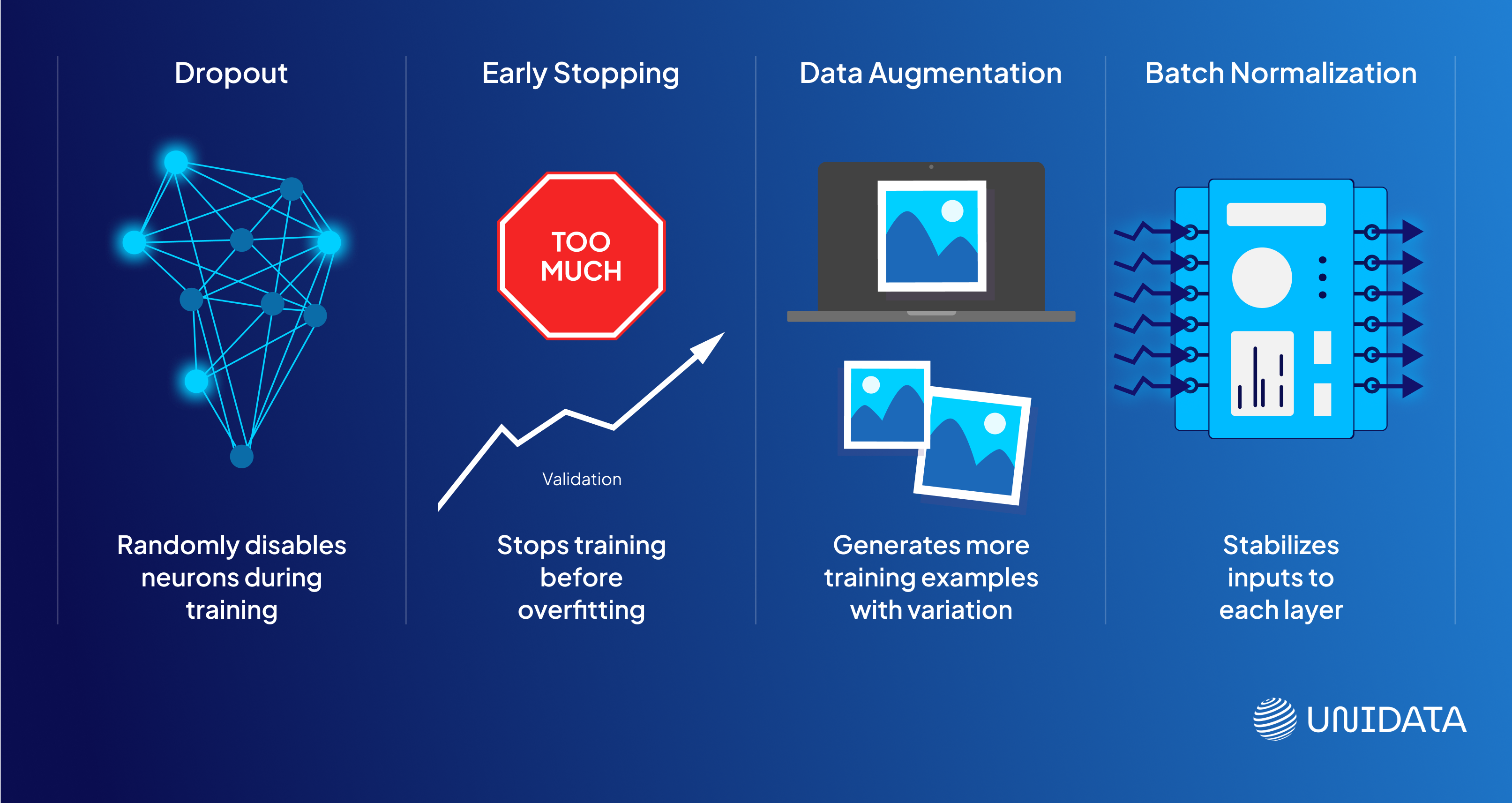
Dropout
Imagine you're training for a group project, but you’re told you can’t always work with the same teammate. Some days Alex is there, some days they’re not. You’re forced to learn to solve problems with different people each time. That’s what Dropout does inside a neural network.
During training, Dropout randomly turns off a fraction of neurons in each layer. This forces the network to learn redundantly across multiple paths, rather than depending too heavily on one. It’s like resilience training—your model gets better at handling uncertainty.
- Common values: Dropout rates between 0.2 and 0.5
- Only used during training, not inference
import tensorflow as tf
from tensorflow.keras.layers import Dense, Dropout

# Add a dense layer with 128 neurons and ReLU activation
model.add(Dense(128, activation='relu'))

# Apply dropout to prevent overfitting (drops 50% of neurons)
model.add(Dropout(0.5))
Early Stopping
Picture someone over-preparing for an exam. They keep studying even after they've nailed the material, and eventually, their performance dips from burnout. Models can do the same—they can keep training until they start learning noise instead of patterns.
Early stopping monitors the model’s performance on a validation set and halts training once that performance stops improving. It’s like an automatic seatbelt for overfitting.
- Reduces unnecessary training
- Avoids overfitting by watching for rising validation loss
- Best used when training deep networks over many epochs
from tensorflow.keras.callbacks import EarlyStopping

# Set up EarlyStopping to monitor validation loss with a patience of 3 epochs
early_stop = EarlyStopping(monitor='val_loss', patience=3)

# Train the model with 20% of data used for validation and apply the callback
model.fit(X_train, y_train, validation_split=0.2, callbacks=[early_stop])
Data Augmentation
In computer vision tasks, you don’t always have millions of images. But you can make it feel like you do. Data augmentation creates new training examples by slightly altering your existing images—flipping, rotating, zooming, or shifting them.
This gives your model a wider view of the world and helps it generalize better.
- Used heavily in image classification and object detection
- Doesn’t actually change the original dataset—it just creates a variation on the fly
from tensorflow.keras.preprocessing.image import ImageDataGenerator

# Create a data generator with rotation, zoom, and horizontal flip for augmentation
datagen = ImageDataGenerator(
    rotation_range=30,
    zoom_range=0.2,
    horizontal_flip=True
)

# Fit the generator to training image data
datagen.fit(X_train_images)
It’s like training your model on a “what-if” version of your dataset: “What if the image is slightly rotated? What if it’s zoomed in?” That flexibility builds stronger pattern recognition.
Batch Normalization
Training a deep neural network is like hiking up a mountain—some paths are smooth, others are chaotic. Batch Normalization smooths out the terrain. It normalizes the inputs to each layer during training so that the network doesn't have to constantly adjust to shifting data distributions.
But here’s the twist—it also has a regularizing side effect. By adding slight noise and controlling internal covariate shifts, batch norm makes the model less sensitive to overfitting.
- Works well with or without Dropout
- Speeds up training
- Reduces the need for other regularization in some cases
from tensorflow.keras.layers import Dense, BatchNormalization

# Add a dense layer followed by batch normalization to stabilize learning
model.add(Dense(128, activation='relu'))
model.add(BatchNormalization())
4. What Are Bias and Variance?
To build a reliable machine learning model, you need to understand why it makes errors. Two of the biggest reasons are bias and variance. Let’s break them down.
Bias: Missing the Mark
Bias happens when a model makes strong assumptions about the data—like trying to fit a straight line to a curve. It's too simple to capture what's really going on. As a result, it can't learn the underlying patterns well, which leads to errors in both the training data and unseen data. This is called underfitting.
High bias = model doesn’t learn enough = poor performance everywhere.
Variance: Overreacting to the Details
Variance happens when a model is too flexible. It picks up on every little detail in the training data—even the random noise. That means it learns the training data very well, but it doesn't perform well on new data because it's too tuned to the specifics of what it has already seen. This is called overfitting.
High variance = model learns too much = great on training, bad on test data.
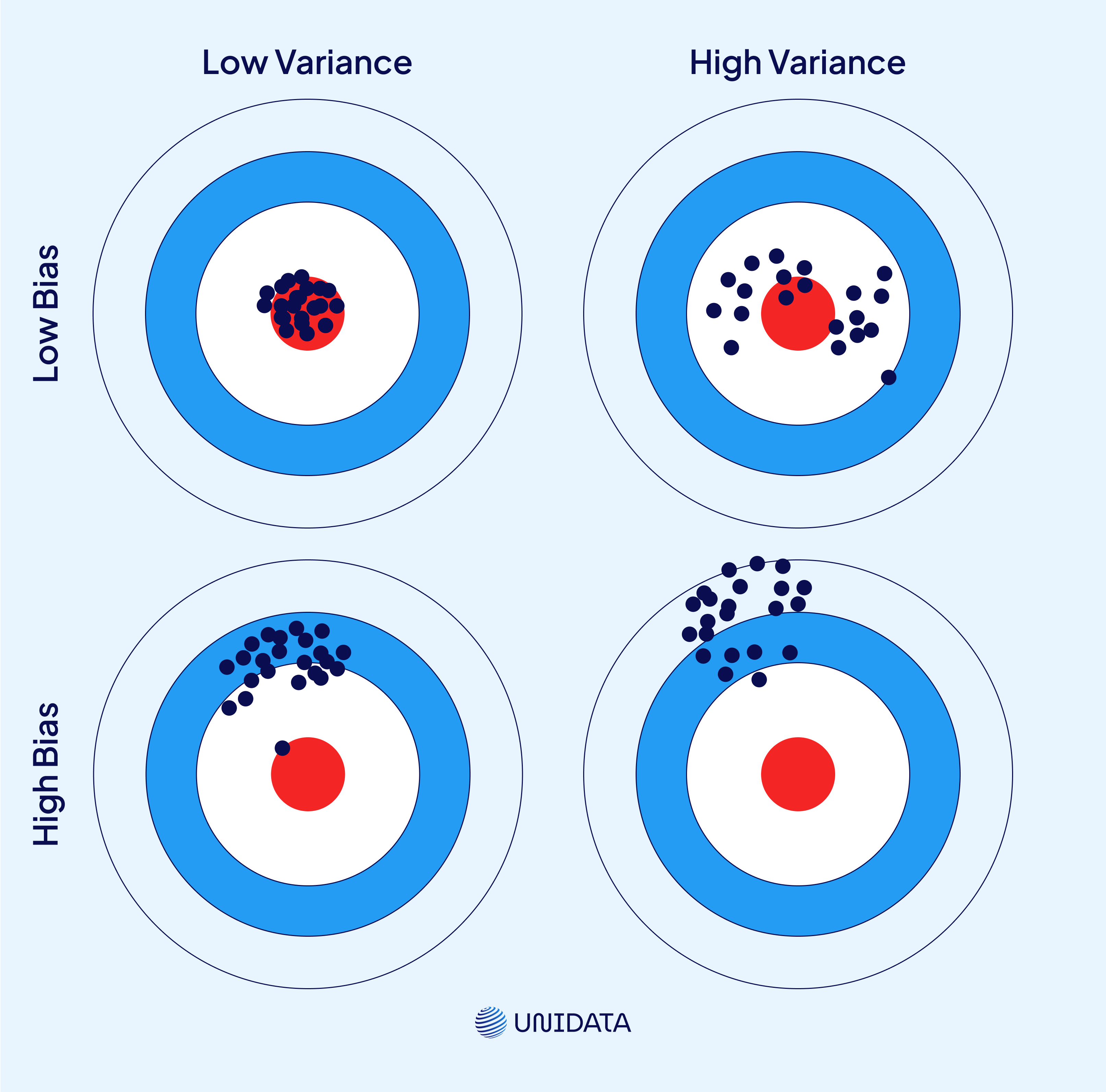
Imagine you're trying to hit the bullseye on a dartboard.
- A high-bias model is like someone who always throws darts in the same wrong direction. The darts land close together but far from the center. Consistent, but consistently off.
- A high-variance model is like someone whose darts are all over the place—some hit close, others are far off, with no clear pattern.
- A good model throws darts that land close to the bullseye and close to each other. That’s what we’re aiming for.
This is what bias and variance look like in action:
| Scenario | Bias | Variance | Typical Result |
|---|---|---|---|
| High Bias | High | Low | Underfitting |
| High Variance | Low | High | Overfitting |
| Balanced | Moderate | Moderate | Good generalization |
The Bias-Variance Tradeoff
Here’s where things get tricky: reducing one usually increases the other.
- If you make your model more complex to reduce bias, it might start overfitting (higher variance).
- If you simplify your model to reduce variance, it might underfit (higher bias).
This is the bias-variance tradeoff. The goal is not to eliminate both, but to balance them. A good model has just enough flexibility to learn meaningful patterns but not so much that it chases random noise.
5. Role of Regularization
So far, we’ve explored how model errors stem from bias and variance, and the delicate balancing act that’s needed to get both under control. But how do we actually guide the model toward that balance?
Regularization works quietly behind the scenes, influencing how the model learns, what patterns it prioritizes, and how far it's willing to go to reduce error. It doesn’t stop the model from learning—but it makes sure that learning stays grounded.
Here’s how it helps:
- It adjusts the model’s objective, asking not just for lower error, but for simpler, more stable solutions.
- It discourages extreme behavior, like overly large weights or hyper-specific decisions that only work for a few cases.
- It reduces sensitivity to outliers and overcomplicated trends.
This balance is especially important when dealing with high-dimensional, messy, or limited datasets—where it’s easy to find patterns that don’t actually hold up in the wild.
A Deep Dive into AI Model Training: Concepts, Techniques, and Best Practices
Learn more
Benefits of Regularization (That You’re Probably Already Relying On)
Regularization isn't just theoretical; it delivers tangible benefits:
Helps Models Generalize, Not Memorize
The real world doesn’t look like your training set—and regularization knows that. It teaches the model to focus on patterns that are likely to show up again, not just the ones it saw once.
That’s exactly how Tesla’s self-driving models avoid tunnel vision. They don’t just learn to drive in ideal conditions—they learn the rules of the road. Regularization helps them adapt whether it’s bright daylight, pouring rain, or an unfamiliar intersection.
Filters Out Noise
When data is noisy or sparse, regularization becomes a model’s best defense. It prevents overreacting to every outlier and keeps learning on solid ground.
At CERN, where particle collisions generate oceans of chaotic data, researchers use regularization to help models stay focused. It keeps them from finding patterns that only exist once and ensures that any signal they detect is actually meaningful.
Stabilizes Learning
If your model is too reactive, small changes in data can throw off predictions. Regularization smooths out that behavior, creating models that are less jumpy and more reliable.
Target’s customer segmentation models depend on that stability. Just because someone bought a random product once doesn’t mean their profile should change overnight. Regularization helps the system resist these tiny tremors and stay consistent over time.
Focuses Attention on What Actually Matters
In high-dimensional data, it’s easy for models to get lost. Regularization keeps them grounded—highlighting the strongest signals and ignoring distracting noise.
That’s how Netflix keeps its recommendations relevant. With millions of users and titles, the model needs to cut through the clutter. Regularization helps it stick to consistent viewing patterns instead of reacting to every late-night anime binge or one-off documentary click.
Wrapping It Up
Regularization is your go-to tool for keeping machine learning models tuned to perfection. Whether predicting market trends, customer behavior, or medical outcomes, regularization ensures your models stay reliable and trustworthy. Remember, a well-regularized model isn't just mathematically appealing—it's practically impactful.
Frequently Asked Questions (FAQ)
Regularization in machine learning is a technique used to reduce overfitting by adding a penalty term to the model’s loss function.
The two main types of regularization in machine learning are L1 regularization (Lasso) and L2 regularization (Ridge). Both add penalties to the loss function but affect model weights differently. L1 regularization shrinks some feature weights to zero, effectively performing feature selection. L2 regularization reduces the magnitude of all weights without eliminating them, leading to more balanced models. Both techniques help control overfitting and improve generalization.
Regularization reduces overfitting by penalizing complex models and discouraging large weights during training. This prevents the model from fitting noise in the data.
Elastic Net regularization combines L1 and L2 regularization to balance feature selection and weight shrinkage. It is especially useful when dealing with correlated features. By introducing a mixing parameter, Elastic Net allows models to both eliminate unimportant features and maintain stability across related variables. This makes it a flexible and powerful approach for complex datasets.
Other regularization techniques include dropout, early stopping, data augmentation, and batch normalization.
- Dropout randomly disables neurons during training to improve robustness.
- Early stopping halts training when performance stops improving.
- Data augmentation increases dataset diversity, and batch normalization stabilizes learning.