Missing Values in Data: What It Is and How to Handle It

Ignoring gaps in data is like baking a cake without sugar — you won’t like the result. These “holes” (blanks, nulls, NaNs) are everywhere in real-world datasets and can hide critical information. 

In this guide, we’ll cover what missing values are, why they matter, and how to handle missing data. You’ll learn about MCAR, MAR, and MNAR, explore deletion vs. imputation, and see techniques from mean substitution and forward fill to linear interpolation, KNN, regression, multiple imputation (MICE). Python code examples and expert tips will help you choose the right approach. Let’s patch these data potholes before your models spin out. 

What Are Missing Values in Data?

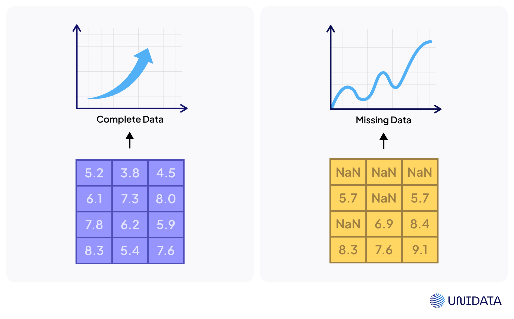
Missing values (or missing data) are points that should exist but don’t. Instead of a value, you see an empty cell or a placeholder like NA or NULL. They appear for many reasons: skipped survey answers, sensor glitches, data entry errors, lost records, or mismatched merges. Whatever the cause, a missing value is information that could have mattered — but isn’t there.

Real-world datasets are rarely complete. Healthcare records may lack lab results for patients who missed a test; e-commerce logs often contain blank fields when customers withhold details. Analysts distinguish observed data (values present) from unobserved or missing ones. A row without gaps is a complete case; any missing field makes it incomplete data. Studies confirm missing values “conceal a valuable piece of information” that can shape outcomes if revealed. 

Why Missing Data Matters

Missing values aren’t just messy — they can break your analysis. Fewer complete cases mean lower statistical power and a higher chance your model misses true patterns. Worse, if missingness relates to hidden trends, results become biased and may lead to invalid conclusions.

From a machine learning angle, many algorithms crash with NaNs. A simple linear regression, for instance, won’t run until missing data are dropped or imputed. Deleting rows might seem easy, but it shrinks your dataset and risks bias unless data are missing completely at random (MCAR). As Nature notes, dropping cases often cuts power and distorts results if missingness ties to outcomes.

Even models that tolerate gaps (like some tree ensembles) lose interpretability and reliability. Research shows models trained on poorly imputed values can yield misleading predictions. The takeaway: missing values in data must be handled deliberately — never ignored. 

Types of Missing Data (MCAR, MAR, MNAR)

Not all missing data are equal. Why values vanish determines how serious the problem is.

Missing Completely At Random (MCAR)

The dream scenario, but rare. Missingness is pure chance, unrelated to the value or any other data. Like a survey where a few people randomly skip a question. Analyses stay unbiased — you just lose sample size. Example: a lab machine glitches and occasionally forgets to record a result.

Missing At Random (MAR)

Far more common. Here, missingness depends on other observed data, not the value itself. Imagine younger respondents skipping income questions. Age predicts who leaves blanks, not income. If you include those observed factors in your model or imputation, bias can be fixed. Ignore MAR, and results skew fast.

Missing Not At Random (MNAR)

The nightmare. Missingness is tied to the missing value itself. Patients with severe symptoms may drop out; low-income respondents may refuse to answer. Here, the absence speaks volumes. MNAR brings heavy bias, and you often can’t spot it from the data alone. Handling it means sensitivity analyses or modeling the missingness process directly.

In practice, analysts often assume MAR — it’s workable, unlike MNAR, and less naive than MCAR. The key is matching your method to the mechanism: MCAR and MAR can be patched with smart fixes, while MNAR demands caution and creativity. 

Deletion Methods for Missing Data

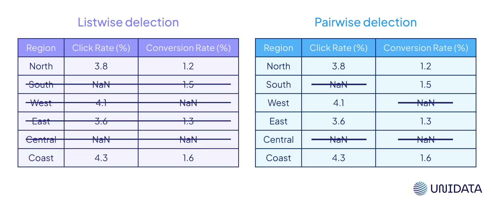
One simple fix is deletion — drop the incomplete data. The classic version is listwise deletion (complete-case analysis): remove any row with a missing value (PMC). Easy, which is why many statistical software packages default to it. The catch? You can lose a lot. If 30% of rows have gaps, you’ve instantly lost 30% of your dataset.

Listwise deletion slashes sample size. If data are MCAR, estimates remain unbiased — though less precise. If not, deletion can distort results. Example: if high-income respondents tend to skip questions, dropping them biases any income analysis. 

Pairwise deletion (available-case analysis) is looser. Instead of cutting entire rows, it uses all data available for each calculation. For example, a correlation between X and Y uses only cases where both are present. This preserves more data but creates inconsistencies: different statistics come from different subsets, and correlation matrices can even fail to be positive-definite. Pairwise deletion can be less biased than listwise if data are MCAR or MAR, but with heavy missingness it quickly becomes messy.

When to delete? If only 1–5% of values are missing and the gaps look random, deletion may be fine (Gartner). Dropping a column is also common if it’s mostly empty (say, 60% missing). But always report what you removed and test the impact: run analyses both ways — deletion vs. imputation. If results shift, missing data is driving outcomes, and a more advanced fix is needed. 

Single Imputation Techniques: Filling in the Blanks

Instead of deleting rows, we often impute missing values — fill gaps with estimated ones. Single imputation means each missing entry gets one replacement. It keeps datasets complete but can add bias if used carelessly.

Mean/Median/Mode 

Replace blanks with the mean, median, or most frequent value. Simple, fast, and keeps sample size intact (Atlan). The drawback: it reduces variance and weakens correlations, often making models look overconfident.

Forward Fill / LOCF 

In time series, missing values are replaced with the last observed one. It maintains continuity but assumes stability, which is often false. Overuse can freeze trends and bias results. Experts advise against LOCF unless the assumption is justified (PMC).

Linear Interpolation 

Fills gaps by connecting known points with straight lines. Works for smooth, gradual changes but misrepresents nonlinear patterns. 

Linear interpolation fills gaps by “drawing a straight line” between the nearest known points.
For example:

Day 1 = 10
Days 2 and 3 = missing
Day 4 = 40

We assume the growth was steady:
Day 2 = 20
Day 3 = 30

In other words, the missing values are estimated as points on a straight line connecting their neighbors. 

Regression Imputation 

Predicts missing values from other features. Preserves relationships but shrinks variability, making estimates too neat. Some implementations add random noise to mimic real variation (PMC). 

​​How It Works

We take the column with missing values — this is our target variable. The remaining features serve as predictors for the regression. We train the model on the rows that have no missing values. Then, for rows with gaps, we feed their predictor values into the model to estimate the missing ones. 

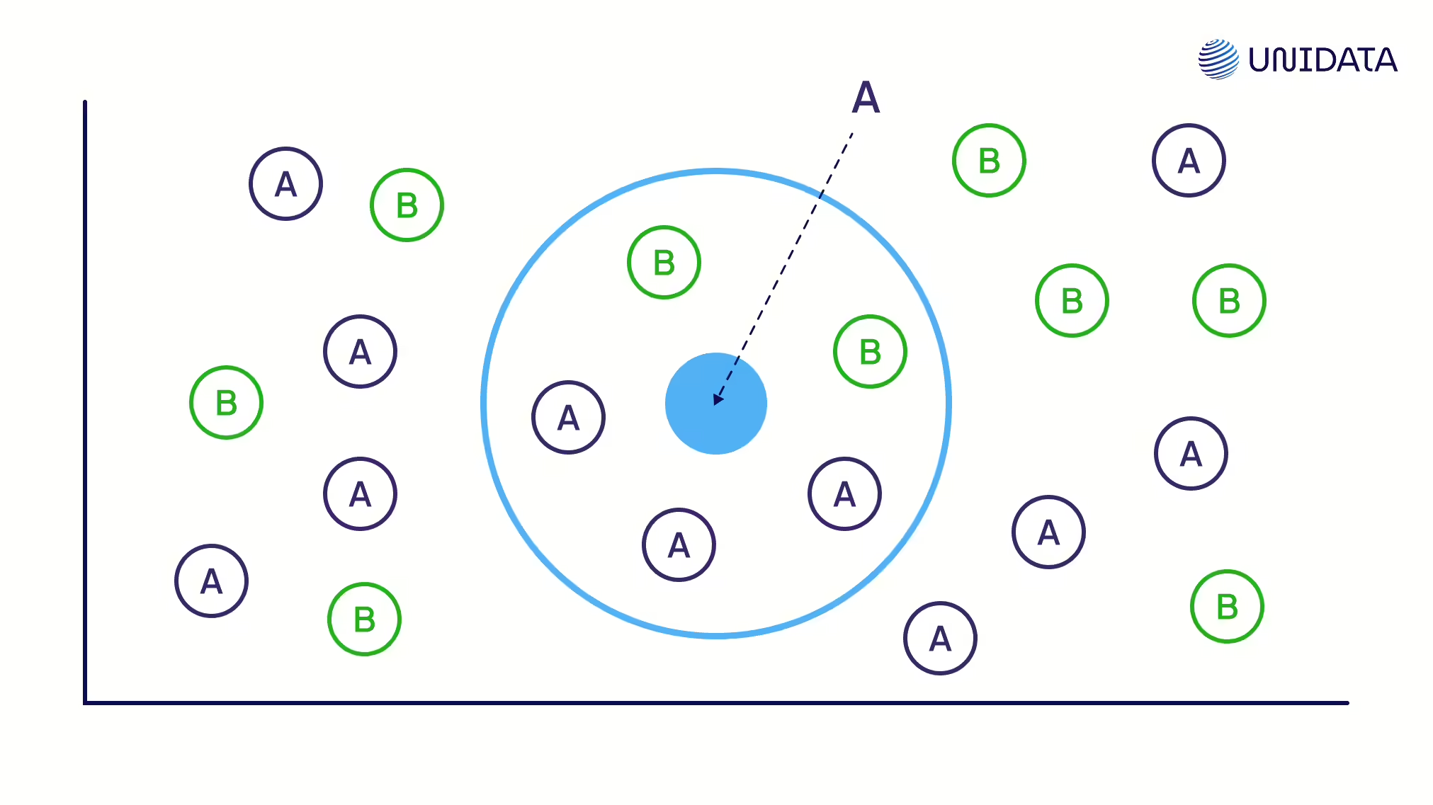
KNN Imputation 

Uses values from the closest data “neighbors.” Good for local patterns but computationally heavy and sensitive to scaling. 

How It Works

For a row with a missing value, we find its k nearest neighbors — the most similar rows based on other features. We take the values of the missing feature from those neighbors. Then we fill the gap with:

• the average of the neighbors’ values (for numerical data), or
  
• the most frequent value (for categorical data). 

Overall, single imputation is like patching holes with one guess — fast and convenient, but it ignores uncertainty. Fine for small gaps; risky for deeper analysis (PMC). 

Multiple Imputation Methods

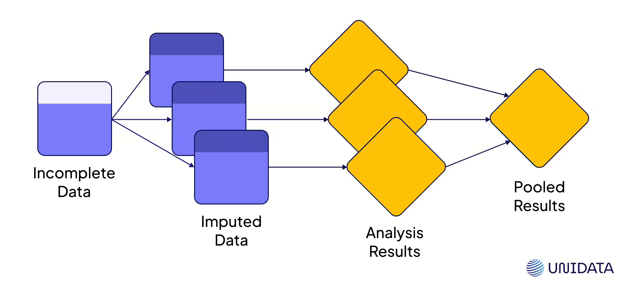
Single imputation is a band-aid. Multiple imputation (MI) is the full treatment. Instead of one guess, MI makes several. It builds multiple “complete” datasets, runs analysis on each, and then blends the results. The benefit? You keep natural variation and get confidence intervals that actually reflect uncertainty (PMC). The workhorse here is MICE (Multiple Imputation by Chained Equations), which fills gaps step by step until the data stabilizes.

Another path is maximum likelihood. Algorithms like EM (Expectation–Maximization) estimate missing values directly from incomplete data. They squeeze every bit of information under MAR. But they’re slow and rely on heavy assumptions. That’s why, in practice, MI often wins — it’s easier, more flexible, and easier to explain. 

When to use what:

• Rich, multivariate data → Iterative Imputer or MissForest.
  
• Sequential data → time-series or state-space models. 

Bottom line: Multiple imputationI remains the gold standard. ML methods are powerful, but they’re sharp tools — use them with care. 

Example: Handling Missing Data in Python

Let’s look at a quick practical example of handling missing values using Python. We’ll demonstrate a couple of simple imputation techniques on a toy dataset using pandas and scikit-learn.

import pandas as pd
import numpy as np
from sklearn.impute import SimpleImputer

# Sample dataset with missing values
data = {
    'Age': [25, np.nan, 30, 32],
    'Salary': [50000, 60000, np.nan, 52000]
}
df = pd.DataFrame(data)
print("Original Data:")
print(df)

In this small DataFrame, the second person’s Age is missing and the third person’s Salary is missing:

Original Data:
    Age   Salary
0  25.0  50000.0
1   NaN  60000.0
2  30.0      NaN
3  32.0  52000.0

1. Impute using Mean: We’ll fill the missing Age with the mean age of the others. For this we can use SimpleImputer from scikit-learn (with strategy="mean") or simply calculate the mean and fill. Let’s use SimpleImputer here:

# 1. Mean imputation for 'Age'
mean_imputer = SimpleImputer(strategy='mean')
df['Age_mean'] = mean_imputer.fit_transform(df[['Age']])

2. Forward Fill: For the Salary, suppose these entries are monthly salaries in sequential order. We can do a forward fill to propagate the last known Salary to the missing entry:

# 2. Forward fill for 'Salary'
df['Salary_ffill'] = df['Salary'].fillna(method='ffill')
print("\nAfter Imputation:")
print(df)

After running these steps, our DataFrame now has new columns showing the imputed values:

After Imputation:
    Age   Salary  Age_mean  Salary_ffill
0  25.0  50000.0      25.0       50000.0
1   NaN  60000.0      29.0       60000.0
2  30.0      NaN      30.0       60000.0
3  32.0  52000.0      32.0       52000.0

We can see that for Age_mean, the missing age (person 1) was filled with 29.0, which is the mean of [25, 30, 32]. For Salary_ffill, the missing salary (person 2) was filled with 60000.0, which is the last observed salary from person 1.

In practice, you would likely choose one technique or another for each column, rather than add new columns as we did for illustration. If we wanted to use a knn imputer or an iterative imputer (MICE), scikit-learn provides KNNImputer and IterativeImputer for those methods. For example:

from sklearn.impute import KNNImputer
knn_imputer = KNNImputer(n_neighbors=2)
df_knn_imputed = pd.DataFrame(
    knn_imputer.fit_transform(df[['Age', 'Salary']]),
    columns=['Age', 'Salary']
)
print("\nKNN Imputed Data:")
print(df_knn_imputed)

This would fill both Age and Salary by looking at the 2 nearest neighbors in the dataset (based on available features). Always remember: after imputation, it’s wise to review the data – ensure that imputed values make sense (e.g., no negative ages, etc.), and possibly mark or flag imputed values if you need to keep track of them for accountability.

Choosing the Right Method to Handle Missing Data

There’s no universal fix. The “best” method depends on why values are missing, the kind of data you have, and what you want to achieve. 

Start with the mechanism. 

• If data is MCAR, and only a few points are missing, simple fixes — like deletion or mean imputation — usually work without bias (PMC).
  
• If it’s MAR, lean on other observed variables. Regression imputation, multiple imputation, or indicator variables can keep bias in check.
  
• If it’s MNAR, there’s no easy cure. You’ll need sensitivity analyses or models that capture the missingness itself.

Match the method to the data. Time-series call for forward fill or interpolation. Numerical features? Mean, median, or regression imputation. Categorical variables? Mode or a simple predictive model. And if your dataset is multivariate, methods like MissForest or iterative imputation shine by exploiting correlations.

Think about your goal. If you need unbiased coefficients and valid p-values, play it safe: multiple imputation or maximum likelihood (PMC). If you only care about predictive power, faster tricks may be fine. Some algorithms, like XGBoost or LightGBM, can even split on “missing” as its own category — no imputation needed.

Check the scale. A tiny 3% gap? Simple fixes will do. A feature that’s 60% empty? Drop it — you’re mostly guessing anyway (Gartner). Always compare results with and without imputation. If your model changes drastically, missing data is driving the story.

Stay alert for bias. Quick fixes reduce variance and can make results look stronger than they are. Multiple imputation or maximum likelihood put the uncertainty back where it belongs. And if you do cut corners, at least be honest about the trade-offs. 

Final Thoughts

Missing values are everywhere. The right way to handle them depends on why they’re missing, the type of data, and your goal.

What you should never do is ignore them. Untreated gaps weaken power, bias results, and mislead models. With the right strategy — whether dropping rows, using simple fills, or applying multiple imputation — you protect the integrity of your analysis.

Handled well, missing values aren’t fatal flaws. They’re just small bumps on the road to reliable insights and stronger machine learning models.