Introduction
Machine learning (ML) is like the brain behind many of today’s smart technologies—helping doctors diagnose diseases, banks detect fraud, and even making self-driving cars possible. But just like how we learn from experience, ML models learn from data. The better and more plentiful the training data, the smarter and more accurate the model becomes.
So, how much data do you need? The answer isn’t one-size-fits-all. It depends on what you’re trying to achieve, the problem is complexity, and the type of model you’re using.
Whether you're just starting or fine-tuning an existing model, understanding your data needs is the first step to success. Let’s dive in!
The Role of Training Data in Machine Learning
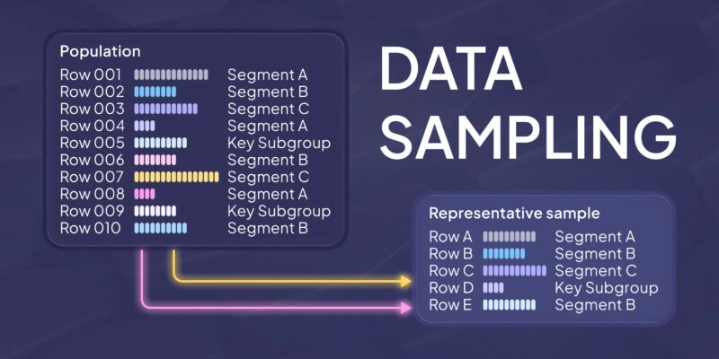
Think of training data as the "textbook" your machine learning model studies from. It’s a collection of examples—each containing input features (like weather data, customer purchases, or images) paired with the correct answers (like "rainy," "fraudulent," or "cat"). By analyzing these examples, the model learns to spot patterns and make its own predictions.

Why does training data matter so much?
- Better learning = smarter predictions – High-quality, diverse data helps your model understand real-world situations, not just memorize examples.
- Avoiding mistakes – Too little data? Your model might miss key patterns (underfitting). Poor-quality data? It could focus on irrelevant noise (overfitting).
- Future-ready AI – A well-trained model adapts to new, unseen data—just like how studying broadly prepares you for unexpected test questions.
How Does the Volume of Training Data Affect Model Performance?
The relationship between the amount of training data and ML model performance can be described by the law of diminishing returns: initial increases in data volume can lead to significant performance gains, but these gains decrease as more data is added.
Here are the key aspects of ML training which are influenced by the amount of data used:
Model complexity and capacity
More data provides a machine learning model with a richer set of examples to learn from and typically improves its ability to generalize to unseen data. This is particularly true for complex models like deep neural networks, which require large datasets to train effectively.
Accuracy and precision
More data can reduce the variance in model predictions, helping a model to discern the underlying patterns more clearly. This significantly reduces the likelihood of anomalies, improving the overall outcomes.
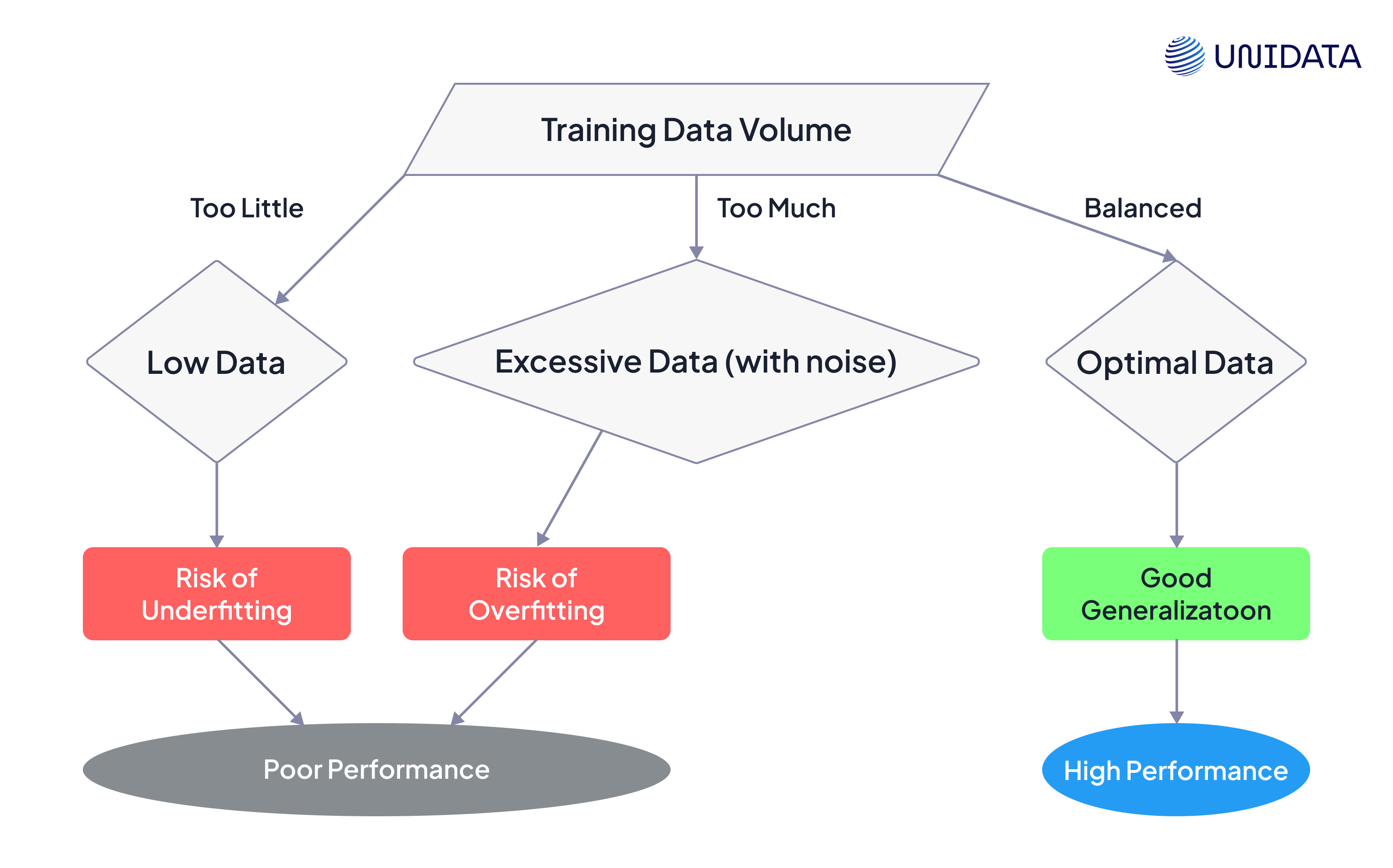
Underfitting vs. Overfitting
With insufficient data, a model may underfit – fail to capture the underlying structure of the data and perform poorly even during the training phase. On the other hand, too much data, particularly if it's noisy or irrelevant, can lead to overfitting: a model may learn the noise in the training set instead of the actual trends, which can result in poor performance on new data.
Factors Influencing the Required Amount of Training Data
Complexity of a ML model
The complexity of a machine learning model depends on the amount and diversity of training data. Simple models, such as linear regressions, require fewer parameters and can function well with less data, especially for tasks with straightforward relationships between features and outcomes.
On the other hand, complex models like neural networks need a wide range of parameters and layers, demanding substantial amounts of data to learn effectively without overfitting. While these intricate models excel at capturing patterns and nonlinear relationships in the data, they require training datasets to encompass the full range of potential variations and interactions within the data features.
Type of ML Problem
Different types of machine learning problems and different approaches to them require varying amounts of data. An analysis of 20 datasets suggests that for classification tasks, training sets between 3,000 and 30,000 samples are often sufficient, depending on the number of classes and features
Supervised Learning
Tasks like classification and regression in this category require a significant amount of labeled data. The data must effectively represent the categories or values that the model intends to predict. For instance, supervised image recognition tasks typically perform well with tens of thousands of labeled images.
Unsupervised Learning
These tasks, such as clustering and dimensionality reduction, don’t rely on labeled outcomes but still require big amounts of data to discover patterns and relationships within the dataset.
Semi-supervised Learning
Acting as a middle ground between supervised and unsupervised learning, this ML approach utilizes both labeled and unlabeled data. When it comes to data volume, semi-supervised learning usually requires less labeled data than fully supervised methods but still benefits from large volumes of unlabeled data to enhance learning accuracy.
Reinforcement Learning
The amount of data needed in reinforcement learning depends on the complexity of the environment and the task. The data is generated through interactions with the environment, and sophisticated tasks require extensive interaction to learn effective strategies.
Deep learning
This is a subset of supervised learning, known for its capacity to handle vast amounts of data. Models like deep neural networks require large datasets to train on due to the high number of parameters and the complexity of the patterns.
Type and Number of Input Features
The number and types of input features also play a role in determining the amount of training data required.
Feature Complexity
When dealing with features like high dimensional data or images, the model needs more data to understand intricate details and nuances.
Number of Features
Having more features typically demands more data to capture their relationships and interactions. However, not all features contribute equally to the model’s performance. Feature selection technique can help reduce the number of features, potentially lowering the required data volume.
Additionally, methods like PCA or feature importance scoring can minimize data requirements by focusing on the important aspects of the data.
Feature Type
Categorical features may need different handling compared to continuous ones, affecting how much data is necessary for model training.
Performance Metrics
The desired level of performance from a machine learning model also impacts the amount of training data needs. Higher accuracy, precision, and recall standards often require more data in critical applications like medical diagnosis or fraud detection. The dataset must be adequate for training the model to consistently achieve or surpass these performance metrics, ensuring reliability in its predictions and classifications.
Finding a Balance Between Quantity and Quality of Training Data
The search for the balance between the amount and quality of training data is an aspect of machine learning that can greatly impact how successful a model is.
Both research and practical experience have shown that increasing the amount of training data typically leads to a better model performance. However, this improvement diminishes after reaching a certain threshold.
High quality data ensures the accurate reflection of the phenomena or processes being modeled, while poor data quality can result in misleading model outcomes. Ensuring data quality typically involves steps like cleaning, normalization, and transformation. This process is essential for mitigating biases and variances in the model that could lead to overfitting or underfitting.

Achieving a balance between quantity and quality is a task that often requires experimentation. While having a vast amount of data can be advantageous, it's crucial to maintain its quality to avoid skewing the training process. In some cases, having less, but highly relevant and well-curated data can lead to better model performance than having big amounts of lower-quality data, as proven by a research on fast adaptation of deep networks.
For instance, in the field of medical imaging, using a smaller set of clear and detailed images can be more beneficial for training a precise model compared to a larger set of noisy and inaccurately labeled images. This concept also applies to other areas in ML – from natural language processing to financial analytics.
Overall, determining the amount of training data should depend on the requirements of the machine learning model, the nature of the task at hand, and the available data resources, while ensuring that data integrity and relevance remain a priority.
Rules and Methods for Determining the Optimal Amount of Data
Certain guidelines can offer valuable insights for determining the amount of training data for your project.
Rule of Thumb (10 times rule)
This is an idea based on a calculation that you need to have at least ten times more data points than the number of features in your model. The rule of thumb, which originated from linear statistical models, serves as a practical starting point but may not fully address the intricacies of modern machine learning, especially in complex high-dimensional spaces typical of deep learning environments.
For instance, while a model with 10 features might perform adequately with 100 data points in a linear setting, a deep learning model with the same number of features could necessitate thousands or even millions of data points.
This visualization compares two common approaches for determining how much training data is needed based on the number of features in a machine learning problem. The blue solid line represents the "10 Times Rule", a traditional guideline for linear models, which suggests that you need roughly 10 data points per feature (e.g., 50 data points for 5 features). In contrast, the red dashed line illustrates the much higher data demands of deep learning models, simulated here at 1,000 data points per feature (e.g., 5,000 data points for 5 features).
The chart highlights how data requirements scale differently between simple and complex models. While linear models (blue line) grow modestly with added features, deep learning (red line) demands exponentially more data. For example, at 10 features, a linear model needs only 100 samples, whereas deep learning requires 10,000—a hundred times more. This divergence becomes even more extreme with higher-dimensional data (e.g., 50 features = 500 vs. 50,000 data points).
The takeaway is that model complexity dramatically impacts data needs: classical statistical methods can work with limited data, but deep learning relies on massive datasets to avoid overfitting and capture intricate patterns. The legend helps distinguish these two scenarios, emphasizing why choosing the right model depends not just on accuracy but also on data availability.
Statistical Power Analysis
Statistical power analysis helps to figure out how much data you need to confidently detect an effect or pattern in an ML model. It balances between finding real results and not mistaking random chance for actual findings.
Statistical power analysis involves understanding the expected size of the effect you're looking for, which can help you decide how much data will be enough to detect this effect reliably. The more significant and less variable the effect you anticipate, the fewer data points you might need. This method balances the need for sufficient data to uncover true effects without collecting more data than necessary.
This chart illustrates the crucial relationship between your dataset size and your model's ability to reliably detect true patterns. The curve shows how detection confidence (statistical power) improves as you add more data samples. At first, each new data point significantly boosts your model's accuracy - this is where the curve rises steeply. However, after a certain point (typically around 2,000-3,000 samples in this example), adding more data provides diminishing returns. The curve flattens, meaning extra samples stop meaningfully improving your model's performance.
The x-axis represents your data volume (number of samples), while the y-axis shows detection confidence on a scale from 0 (no confidence) to 1 (absolute certainty). The sweet spot occurs where the curve begins to level off - this tells you the optimal amount of data to collect before you're just wasting resources. Hover over any point to see the exact power percentage at different sample sizes, helping you make informed decisions about your data collection strategy.
Empirical Evaluation
Studying how model performance changes with varying amounts of training data can offer valuable insights. Beginning with smaller datasets and gradually increasing the amount of data enables observation of shifts in model accuracy, risks of overfitting, and consistency in learning. This step-by-step method, often paired with cross-validation, aids in grasping the model's learning progression and pinpointing the stage where adding more data no longer enhances performance significantly.
These rules and methods don’t work in isolation but rather complement each other to provide a holistic view of the data needs. Data scientists often combine these approaches, adjusting their strategies based on the specific characteristics of their model, the data available, and the task requirements.
This chart shows how a model’s performance changes as more training data is added. The blue line represents model accuracy, which improves as the amount of training data increases. Initially, the accuracy increases quickly, but the rate of improvement slows down as more data is added, eventually plateauing at higher data sizes. This indicates that adding more data beyond a certain point has a diminishing effect on improving the model’s performance.
The red dashed line shows the risk of overfitting, which occurs when the model becomes too tailored to the training data and struggles to generalize to new data. With smaller datasets, the model is more likely to overfit, but as more data is introduced, the risk decreases. However, once the data size becomes large enough, the model may start to fit too closely to rare patterns in the data, slightly increasing the risk of overfitting, though the impact on performance remains minimal.
In the initial phase with small datasets, the model’s accuracy is low, and the overfitting risk is high. As the dataset grows, the model’s accuracy improves, and the risk of overfitting decreases. Once the data size reaches a certain point, the model’s accuracy plateaus, and while overfitting risk may increase slightly, further increases in data have minimal effect on performance.
Strategies for Dealing with Limited Data
When data is scarce, ML practitioners must find ways to maximize the utility of the available information. These strategies help in training more robust models, even with limited data.
Data Augmentation
By adding synthetically generated examples or transformations to the training data, practitioners can improve model robustness and prediction accuracy.
It involves applying various transformations to the existing data to create new variation samples.
In Image Processing
In this field, common augmentation techniques include rotation, scaling, cropping, flipping, and color adjustment. Via these data transformations, models can learn from a more comprehensive set of visual features and improve their generalization capabilities.
- Rotation: Rotating images by random degrees (e.g., 15°, 45°, etc.) to allow the model to learn rotational invariance. For example, rotating a picture of a cat to simulate how it would appear from different angles.
- Scaling: Resizing an image to simulate different distances from the camera or zoom levels. This helps the model to learn to recognize objects at various scales.
- Cropping: Randomly cropping parts of the image. This can be useful for simulating different zoom levels or focusing on parts of the image.
- Flipping: Horizontal or vertical flipping of images to introduce mirror-image variations, which is especially useful for datasets where objects may appear in different orientations. • Color Adjustment: Changing the brightness, contrast, saturation, or hue of the image to simulate various lighting conditions. For instance, adjusting the brightness to simulate sunlight or low-light environments.
In NLP
In Natural Language Processing, augmentation methods might include synonym replacement, back-translation, and sentence shuffling. By expanding the linguistic diversity of the text data, practitioners aid the model in understanding language nuances better.
- Synonym Replacement: Replacing words with their synonyms to introduce linguistic diversity while preserving the sentence’s meaning. For example, “happy” can be replaced with “joyful,” “elated,” or “content.”
- Back-Translation: Translating the sentence to another language (e.g., English to French) and then translating it back to the original language. This introduces slight rephrasing of sentences, making the model more robust to different phrasings. • Sentence Shuffling: Shuffling the order of sentences or clauses within a document or paragraph. This can help the model learn to understand relationships between sentences in various contexts.
In Audio Processing
When augmenting audio data, techniques like adding noise, changing pitch, speed variation, and time stretching are used. Machine learning models, trained with this data, become more robust to variations in sound, which is especially useful in speech recognition tasks.
In addition, the recent advancements in data augmentation methods such as generative adversarial networks (GANs) have enabled the creation of realistic data samples that blur the line between artificial and real-world datasets. Augmentation methods based on GANs have proven the ability to expand the diversity of training datasets.
- Adding Noise: Introducing background noise, such as static or white noise, to simulate real-world conditions where the audio is not always clear. This helps speech recognition models become more robust in noisy environments.
- Pitch Shifting: Modifying the pitch of an audio signal. This could involve making a speech sound higher or lower in pitch, which simulates different speakers or recording conditions.
- Speed Variation: Altering the speed (tempo) of the audio without changing the pitch. This can simulate different speaking rates in speech recognition systems. • Time Stretching: Stretching or compressing the audio without affecting its pitch. This helps the model become more invariant to changes in the duration of sounds or speech.
Transfer Learning
Transfer learning refers to a technique where a model, created for one task, is repurposed as a starting point for another task. This method utilizes the knowledge acquired during the training of the original model to enhance the efficiency and performance of the second model, typically requiring less data.
Examples:
- Image Classification: A model pre-trained on ImageNet (which contains millions of labeled images) can be fine-tuned for a medical imaging task (e.g., detecting tumors in X-rays) with a much smaller dataset. Instead of training from scratch, the model already understands basic features like edges, textures, and shapes, making it more efficient.
- Natural Language Processing (NLP): BERT, a language model pre-trained on billions of words, can be adapted for sentiment analysis on customer reviews with just thousands of labeled examples. The model retains its understanding of grammar and semantics, requiring only minor adjustments for the new task.
- Autonomous Driving: A neural network trained on general object detection (e.g., identifying cars and pedestrians in street images) can be fine-tuned for specialized tasks like detecting construction zones or traffic signs in a new dataset.
In many instances, models are initially trained on extensive datasets like ImageNet for tasks such as image classification or BERT for natural language processing. For example, models like BERT require vast amounts of text data – over 3 billion words – for pre-training. These models can be fine-tuned on smaller, more specific datasets, enabling deep learning advantages even with limited data availability.
Transfer learning often entails leveraging features learned from the task (e.g. edge detection in images or semantic comprehension in text) and applying them to a new, related problem.
This strategy proves effective by enabling the transfer of learned patterns or features that're often applicable across tasks thereby diminishing the necessity for substantial amounts of task specific data.
Regularization Techniques
Regularization techniques are used to prevent overfitting. These methods adjust the learning process to simplify the model, ensuring it can effectively generalize to new data.
L1 and L2 regularization methods
The L1 and L2 approaches are used to prevent overfitting.
The L1 regularization, or Lasso regularization, adds a penalty to the sum of the absolute values of the model coefficients. Some coefficients may be valued at exactly zero, effectively removing those features from the model. It highlights the most important features and gets rid of unnecessary ones.
Example: In predicting house prices, if features like "distance to nearest park" and "number of nearby schools" are irrelevant, L1 may zero them out, keeping only key factors like "square footage" and "location."
The L2 regularization, or Ridge regularization, adds a penalty to the sum of the square of the model coefficients. This doesn’t necessarily reduce coefficients to zero but shrinks them. This way, all features are retained but their influence on the model is balanced. L2 is good for dealing with multicollinearity (when two or more features are highly correlated) and for improving model prediction.
Example: In a model predicting stock prices, if two features (e.g., "trading volume" and "market sentiment") are highly correlated, L2 ensures neither dominates, balancing their influence.
Dropout
Widely employed in neural networks, this method randomly excludes a subset of features or activations during training. This compels the model to not overly rely on any single feature and instead discover more general patterns within the data.
Example: In a neural network classifying handwritten digits, dropout prevents over-reliance on specific pixel patterns, improving generalization to different handwriting styles.
Elastic Net Regularization
This approach combines the penalties of L1 and L2 regularization. It benefits from both L1’s feature selection trait and L2’s smoothing effects. In a scenario where a machine learning model predicts financial trends, Elastic Net can aid in handling financial indicators (some of which may have strong correlations) by balancing each feature's contribution to prevent overfitting on limited training data.
Example: In financial trend prediction, if some economic indicators (e.g., "inflation rate" and "GDP growth") are correlated, Elastic Net can reduce overfitting while keeping useful predictors.
Tools for Assessing and Increasing Data Volumes
Several tools and resources can aid in assessing and managing the volume and quality of training data.
| Category | Tools | Key Features | Links |
|---|---|---|---|
| Sample Size Calculators | Power and Sample Size (PASS) | • Estimates required sample size for studies • Adjusts for power, effect size, and significance thresholds | PASS Website |
| G*Power | • Free, user-friendly tool for statistical power analysis | G*Power | |
| Data Profiling Software | Pandas Profiling | • Generates interactive EDA reports. • Summarizes distributions, and correlations | Pandas Profiling Docs |
| Informatica | • Enterprise-grade data profiling and cleansing | Informatica | |
| Machine Learning Frameworks | TensorFlow / PyTorch | • Built-in data visualization (e.g., TensorBoard) • Supports large-scale data pipelines | TensorFlow / PyTorch |
| Scikit-learn | • Tools for cross-validation, feature importance. • Helps estimate data needs. | Scikit-learn | |
| Data Augmentation Libraries | Augmentor (Images) | • Rotations, flips, distortions for image data | Augmentor GitHub |
| imgaug | • Supports diverse augmentations (e.g., noise, blur) | imgaug GitHub | |
| Keras Preprocessing Layers | • On-the-fly augmentation for text/tabular data | Keras Docs | |
| Cloud-Based Data Services | AWS (S3, SageMaker) | • Scalable storage (S3) • AutoML and data labeling tools (SageMaker) | AWS SageMaker |
| Google Cloud (BigQuery, Vertex AI) | • BigQuery for SQL-based analysis • Vertex AI for automated data labeling | Vertex AI | |
| Azure (Blob Storage, ML Studio) | • Data versioning and pipelines • Integrated ML workflows | Azure ML Studio |
Case Studies: Successful Projects with Limited Data
In ML, there are numerous examples where innovative approaches have led to successful projects, even with limited data.
Disease Prediction with Clinical Data
A study conducted by Enlitic focused on classifying abnormalities from clinical radiology reports, particularly chest x-ray reports. The project was successful in using small amounts of data: contrary to common belief, effective medical natural language processing models can be trained with relatively few labeled examples.
The deep learning models were able to make use of the training data, outperforming state-of-the-art rule-based systems significantly with just a few thousand reports.
The study found that the performance between models trained on 6,000 to 30,000 reports was comparably high, demonstrating that a smaller dataset can still bring outstanding results.
Few-Shot Learning for Natural Language Understanding
Recently, a few-shot learning approach was introduced that significantly reduces the amount of labeled data required for training machine learning models, particularly in natural language understanding tasks.
A recent project introduced the T5 (Text-to-Text Transfer Transformer) model, which could perform a variety of tasks, including translation, classification, and question answering, with very few training examples.
The model was pre-trained on a large text corpus and then fine-tuned on specific tasks with limited labeled data. The model's architecture allowed for flexible adaptation to different tasks with minimal task-specific data.
This demonstrates that extensive pre-training on large datasets combined with few-shot learning on task-specific datasets can lead to high-performing models even with limited labeled data.
Conclusion
The amount of training data required for machine learning projects is a nuanced issue that depends on various factors, including the complexity of the model, the specificities of the task, and the quality of the data. While having a large dataset is generally beneficial, there are real-life case studies and examples which prove that with the right techniques and approaches, limited data can also lead to successful outcomes.