If you want to know whether a batch of cookies came out right, you do not eat the whole box. You take a few from different corners, taste them, and make a call. Data sampling works the same way: you inspect a subset so you can reason about the whole without paying the full cost.
What is data sampling?
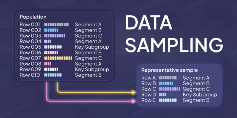
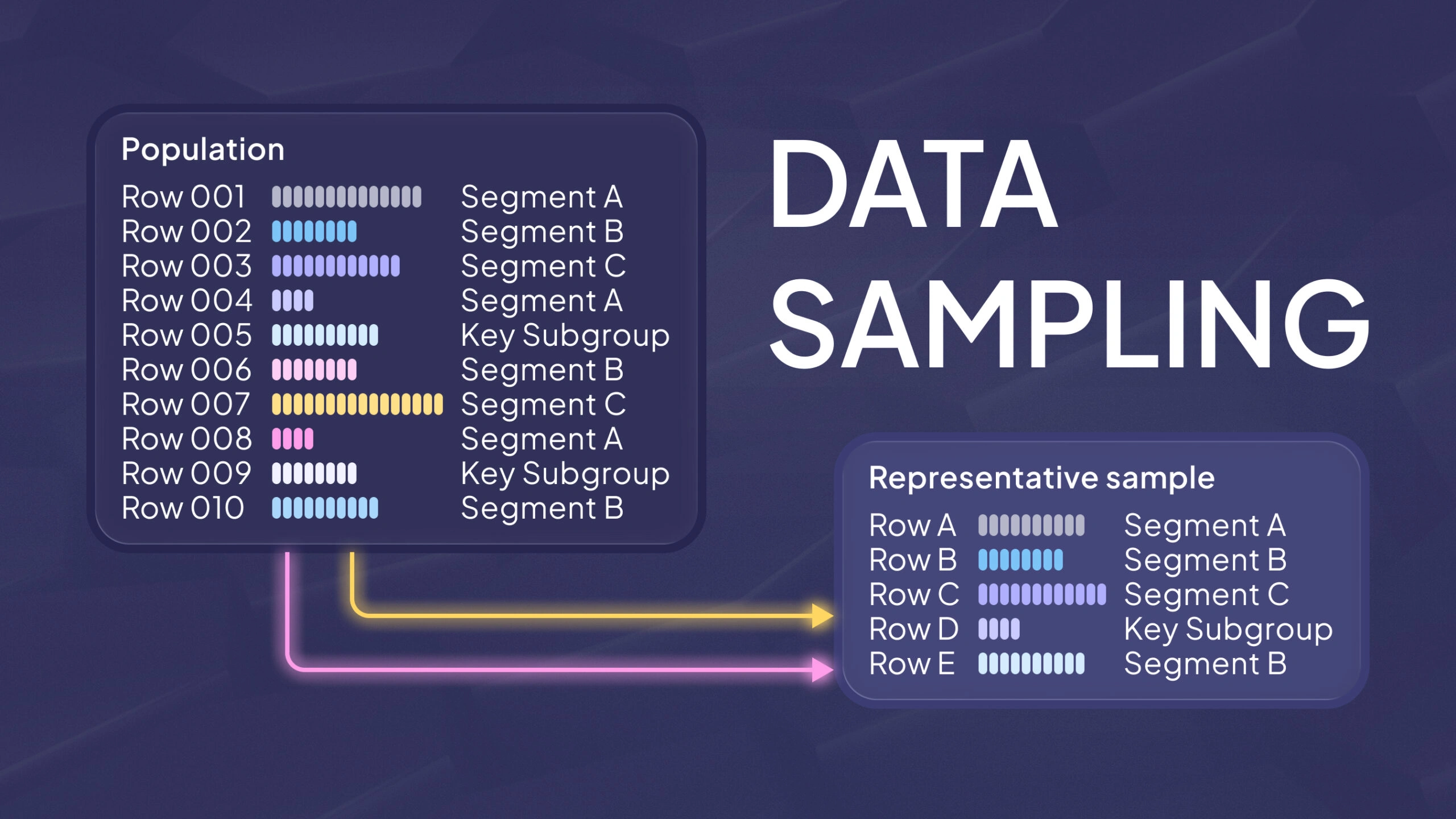
Data sampling is the practice of selecting a subset of observations from a larger population (or dataset) so you can analyze, test, or model without processing everything. The population is the full set you care about. The sample is what you actually observe.
A good sample is not “small.” A good sample is representative. It reflects the patterns that matter in the population, including rare but important cases. It also avoids systematic over- or under-representation of a group.
Sampling shows up across common workflows, and the goal shifts slightly each time:
- Analytics: you query a subset of events to get faster answers, then sanity-check that the slice behaves like the whole.
- Quality control: you inspect a subset of units from a production run to estimate defect rates without stopping the line.
- Surveys: you ask a subset of people and infer what the broader population is likely to think or do.
- Machine learning: you create training and evaluation subsets and want them to match real deployment data.
The shared theme is speed with accountability. You reduce cost, but you keep a clear link to what the results are meant to represent.
Why does data sampling matter?
Sampling matters because full-population analysis is often slow, expensive, or impossible. But sampling is not only a performance trick. It is also how statistical inference works. You use a sample to estimate population parameters like means, proportions, and error rates, and to express uncertainty around those estimates.
Sampling also forces you to define scope. If you cannot define the population and the sampling frame, you cannot defend your conclusions. The sampling frame is the actual list, table, or stream you draw from. Frames are rarely perfect. If the frame misses part of the population, you can get biased results even with “random” selection.
In ML projects, this becomes a deployment risk. A model can look accurate on the data you sampled, then fail on users or conditions your sampling frame did not capture. Sampling does not just shape your analysis. It shapes what you think reality looks like.
How data sampling works
A practical sampling workflow is short enough to run often, but strict enough to be repeatable. The steps below are the backbone.
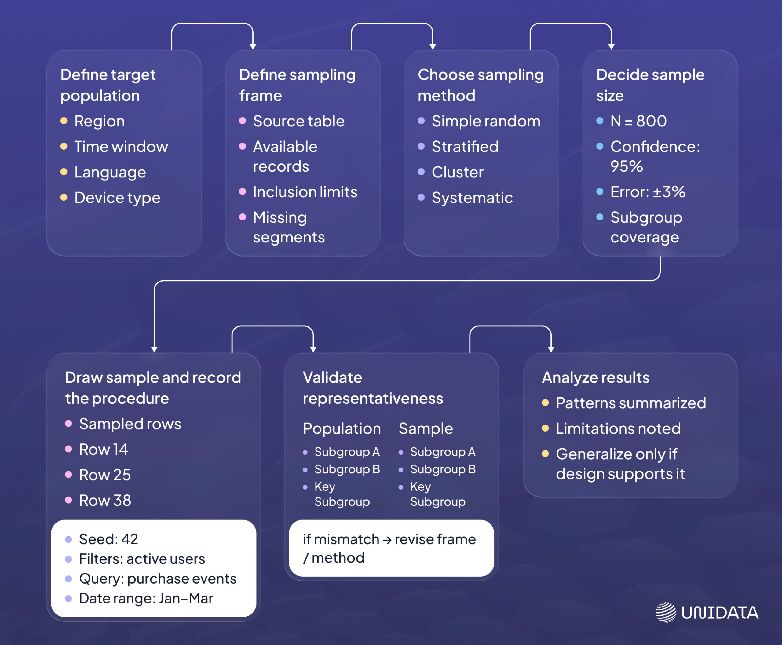
- Define the target population. State what is in scope. Include time window, geography, language, device type, and label space if relevant.
- Define the sampling frame. Identify the table, stream, or process you will sample from. Note what the frame might miss.
- Choose a sampling method. Probability methods support inference. Non-probability methods can speed exploration, with limits.
- Decide sample size. Tie it to the goal: estimation precision, hypothesis testing, model evaluation, or a fixed budget.
- Draw the sample and record the procedure. Save the seed, query, filters, and date range. Reproducibility is part of correctness.
- Validate representativeness. Compare key distributions between sample and full data (or a trusted benchmark). Investigate mismatches.
- Analyze, then generalize carefully. State what the sample supports, and what it does not.
Many teams skip step 6. That is where sampling turns into accidental cherry-picking. A fast sample is still a decision. It needs a quick check before you trust it.
Probability sampling methods
Probability sampling means every unit in the frame has a known, non-zero chance of selection. This matters when you want to estimate population values and reason about uncertainty. If selection chances are known, you can use standard statistical tools more safely.
The choice between methods is usually driven by one question: are you sampling individual rows directly, or are you constrained by how the data is collected and stored?
Simple random sampling
Each observation has the same chance of selection. This is a strong default when the population is fairly homogeneous and you can randomize reliably.
Use it for quick EDA on a large table or for a baseline label-quality audit. The main caveat is practical: truly random selection can be hard if your data is partitioned, streamed, or time-ordered. If the mechanics of retrieval are not neutral, the sample may not be as random as it looks.
Systematic sampling
You pick every k-th unit after a random start, such as every 100th record. It is easy to implement in operational settings, especially when data arrives as an ordered stream.
The main caveat is periodic structure. If your data has cycles that align with k, systematic sampling can distort the sample. Logs that spike on a schedule or batches written in fixed chunks are common sources of this problem. If you suspect periodicity, treat systematic sampling as a convenience method and validate representativeness.
Stratified sampling
You split the population into strata (groups) and sample within each stratum. This is a practical way to avoid the “we missed the minority class because it is only 1%” problem.
n classification, stratified splits help preserve label proportions between train and test. The main caveat is that you must define strata correctly. If the stratification variable is wrong or too coarse, you can still miss the real sources of variation.
Cluster sampling
You sample clusters, then sample within them, or take all units inside chosen clusters. This is often cheaper than sampling individuals directly, especially when the population is naturally grouped.
Use it when collection or access costs are tied to groups, not individual items. The main caveat is correlation within clusters. Observations inside a cluster can be similar, so the effective sample size can be smaller than the raw row count. If you ignore that, you can become overconfident in results.
Multi-Stage Sampling
You combine sampling methods across successive stages — for example, selecting regions first, then households, then individual respondents. This approach is standard in large-scale surveys and field studies where sampling frames are naturally hierarchical.
Use multi-stage sampling when direct selection from a single, clean list is not feasible. The key caveat is compounding complexity: each stage introduces design decisions that can affect representativeness. Rigorous documentation matters more here than it does with simple random sampling.
Non-probability sampling methods
Non-probability sampling means selection chances are unknown. These methods can still be useful, especially early in a project, but they are weaker when you need population claims. They tend to answer “what is in this subset?” better than “what is true in the population?”
Convenience sampling
You take what is easiest to access. It is fast, and it is risky. The sample may reflect your collection pipeline more than your users. Use convenience samples for quick debugging and early exploration.
Quota sampling
You set targets for certain groups, such as 50% mobile and 50% desktop, but choose units non-randomly. It can improve surface-level balance.
The main caveat is bias inside each quota. You can still over-sample “easy” cases within the group, which keeps results biased even though the top-line mix looks balanced.
Purposive (judgment) sampling
You select cases that are information-rich for a specific question, such as hard negatives, edge cases, or known failure modes. This is strong for diagnosis.
The main caveat is measurement. It is not a defensible way to estimate overall error rates, because you intentionally distort the sample toward interesting failures. Keep purposive samples separate from evaluation samples.
Snowball sampling
Participants recruit other participants. This can help when the population is hard to reach and the frame is incomplete.
The main caveat is over-representation of connected communities. The method tends to stay within social clusters, which can skew results.
Choosing between probability and non-probability sampling
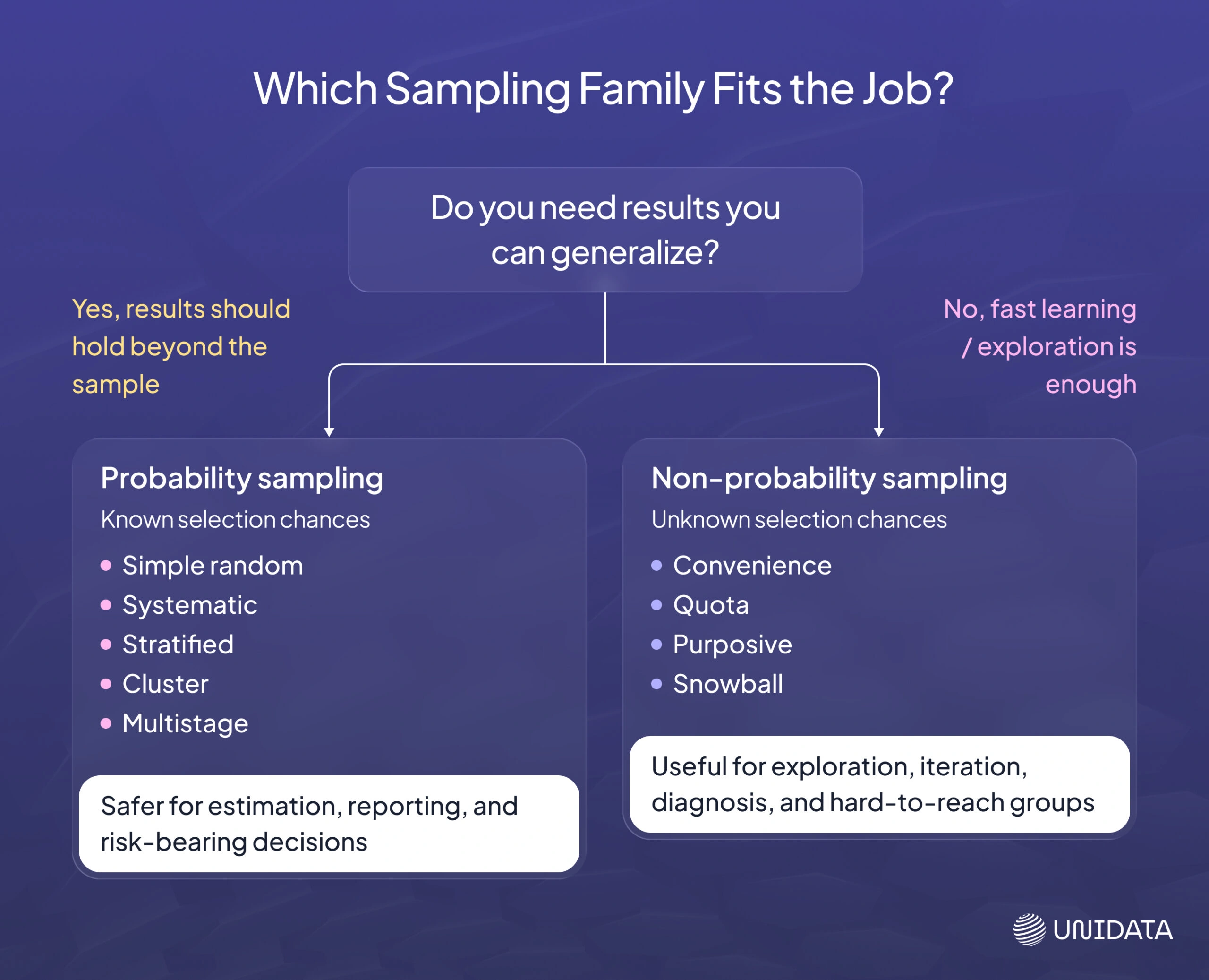
Choose based on what you need to be true about the output.
If your goal is fast learning and iteration, non-probability sampling can be fine, as long as you label it as exploratory and do not treat the numbers as population estimates.
If your goal is estimation, reporting, or risk-bearing decisions, probability sampling is the safer default. Known selection chances give you a clearer path to defensible conclusions, and they make representativeness checks easier to interpret.
When you are unsure, split the work: keep one probability-based sample for measurement, and use targeted non-probability samples for debugging and edge-case discovery.
How to determine sample size
There is no universal “right” $n$. Sample size depends on what you are trying to estimate, how precise you need the estimate to be, how much the population varies, and what your practical budget allows.
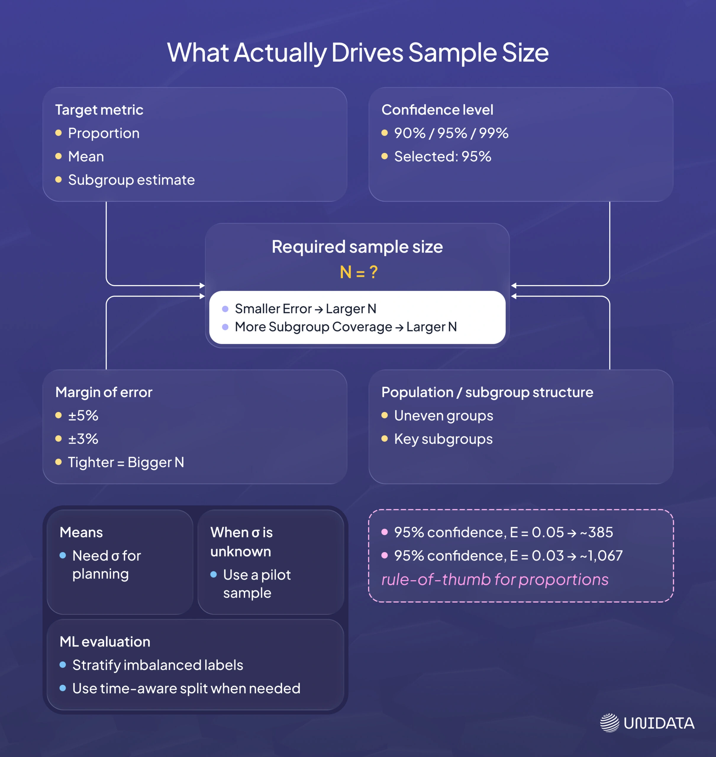
Start by naming the output you want. Once the target is clear, you can pick a confidence level and an error tolerance, then compute a starting sample size. After that, you can adjust based on constraints like finite population size, subgroup coverage, or time windows.
Sample size for a population proportion
When the quantity you want is a proportion (a rate, fraction, or percentage), a commonly used large-sample relationship is:
$$ n = \frac{z^{2}\,p\,(1-p)}{E^{2}} $$Here is what each term means in practical work:
- $$p$$ is your estimated proportion. If you are auditing labels, $$p$$ could be your expected mislabel rate.
- $$E$$ is your desired margin of error, expressed as a proportion. For example, $$E = 0.05$$ means you want your estimate within $$±5$$ percentage points.
- $$z$$ is the critical value for your chosen confidence level. OpenStax: Confidence Interval (Known σ or Large n)
If you do not have a prior estimate for $$p$$, using $$p = 0.5$$ is conservative because it maximizes $$p(1 - p)$$, which produces the largest required sample size. That gives you a safe upper bound for planning.
Common $$z$$ values include 1.645 for 90% confidence and 1.96 for 95% confidence. OpenStax: Confidence Interval (Known σ or Large n)
Quick reference for proportions
The table below assumes $$p = 0.5$$ and uses the formula above.
| Confidence level | z value | Margin of error E | Required n (approx.) |
|---|---|---|---|
| 95% | 1.96 | 0.05 | 385 |
| 95% | 1.96 | 0.03 | 1,067 |
The smaller you make $$E$$, the faster the required $$n$$ grows. OpenStax: Practice Tests (Example sample size calculations)
Finite population correction
The formulas above are often used as if the population is effectively “large.” If you are sampling without replacement from a finite population, and your sample is a meaningful fraction of that population, the finite population correction (FPC) adjusts uncertainty. A common form is:
$$ \mathrm{FPC}=\sqrt{\frac{N-n}{N-1}} $$OpenStax: Finite Population Correction Factor
- $$N$$ is the population size (the total number of individuals or items in the entire group).
- $$n$$ is the sample size (the number of observations or data points collected from the population).
In practice, if your sample is a tiny fraction of the population, the correction is close to 1 and often ignored. If you are sampling a meaningful chunk, ignoring it can overstate uncertainty.
Sample size for a population mean
When the quantity you want is a mean, a commonly used relationship is:
$$ n=\left(\frac{z\,\sigma}{\mathrm{EBM}}\right)^{2} $$OpenStax: Confidence Interval (Known σ or Large n)
- $$\sigma$$ is the population standard deviation (or a prior estimate).
- $$EBM$$ is the error bound for the mean, meaning how close you want your estimate to be.
- $$z$$ is tied to the confidence level, the same way it is for proportions.
This is where real projects often hit a practical issue: $$\sigma$$ is usually unknown at the start. A common approach is to run a pilot sample to estimate variability, then compute a more realistic $$n$$. If a pilot is not feasible, teams use conservative assumptions to avoid under-sampling.
Sample size in ML evaluation
In supervised ML, you often evaluate metrics such as accuracy, $$F1$$, or error rate. The core idea still applies: with fewer examples, your estimates are less stable. This is especially visible when classes are rare, because a test set can be “large” overall but still contain very few examples of the cases you most care about.
Two practical rules from the sampling perspective often matter more than a single formula:
- Stratify splits by label when classes are imbalanced, so every class appears in each split.
- Treat time as a first-class variable. If you have drift, a random split can overstate performance. Use time-based splits when deployment is future-facing.
Once you have a sample size plan, the next question is whether your sampling process introduces random variability, systematic bias, or both.
Sampling error vs sampling bias
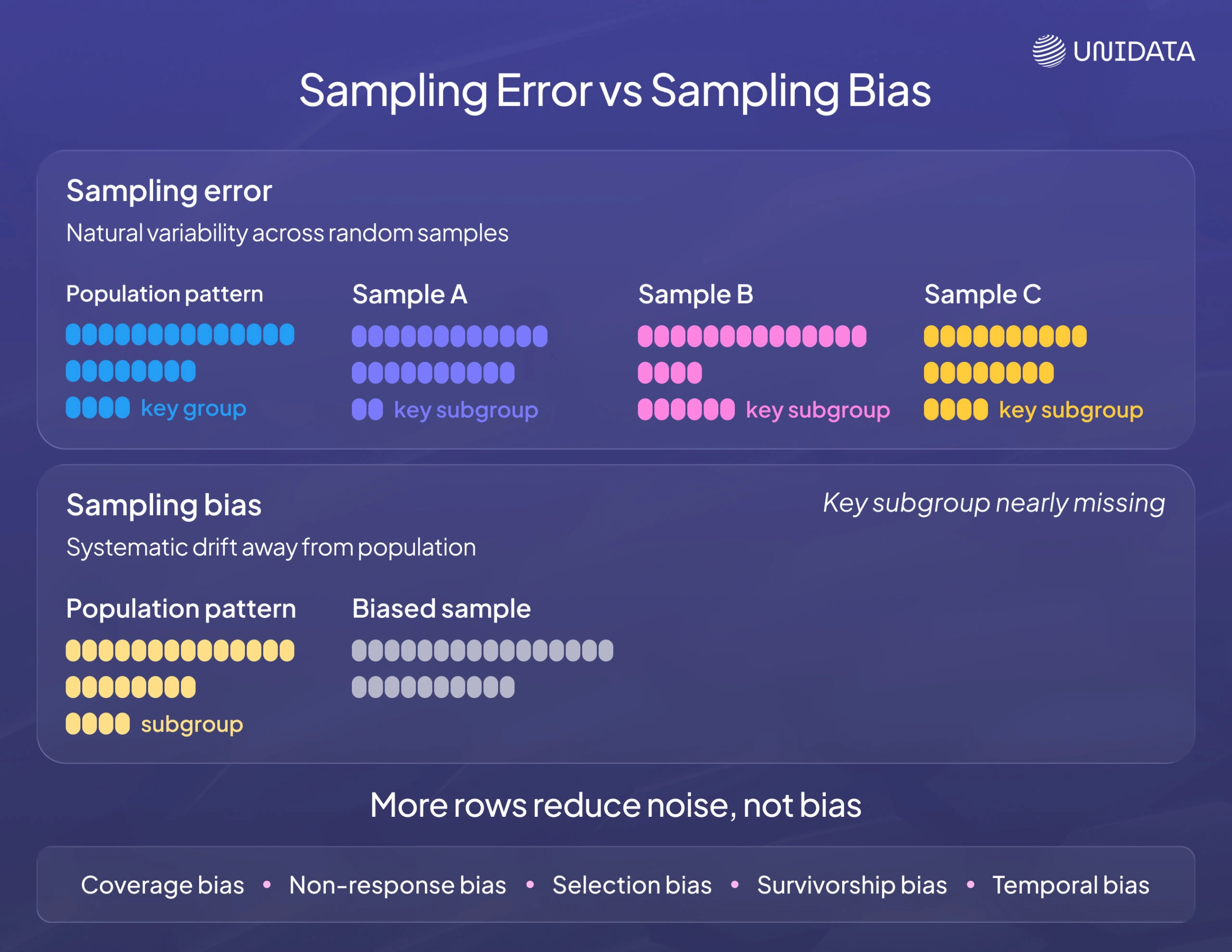
Sampling error is the natural variability you get because you observed a subset rather than the full population. If you draw a different random sample, you will get a slightly different estimate.
Sampling bias is systematic. It happens when the sampling process tilts the sample away from the population, so your estimate is wrong in the same direction over and over.
A large biased sample can be worse than a smaller unbiased sample. Bias does not shrink just because you collect more rows.
Common sources of bias (and what to do about them)
- Coverage bias (frame mismatch): parts of the population are missing from the frame (users without logged-in IDs; devices blocked by tracking). Fix the frame or state the limitation.
- Non-response bias: people or cases that do not respond differ from those that do. Use follow-ups, incentives, or weighting where appropriate.
- Selection bias: you sample “easy” cases (clean logs, happy-path flows) and miss failures. Make failure discovery part of your sampling plan.
- Temporal bias: you sample a convenient time window and treat it as typical. Sample across seasons, releases, and demand cycles.
Real-world sampling examples
Case study 1: Clinical trials (medical research)
Clinical trials often cannot measure outcomes for everyone who might benefit from a treatment. Sampling shows up as participant recruitment and random assignment.
This is an example of “match the population you care about.” If a trial under-represents groups that will use the treatment, the results may not generalize well. Randomization helps manage confounding inside the sample. Representativeness supports external validity.
Case study 3: Market research and polling
Polling is a classic sampling problem: you ask a few to learn about many. The design goal is representativeness, and the communication goal is uncertainty.
In practice, random sampling is often combined with weighting and careful fieldwork to manage who responds and how reachable subgroups are.
Practical sampling tools (Python, R, and SQL)
Sampling is only as good as the implementation. Here are common, reliable building blocks.
Python: pandas
For in-memory tabular data, DataFrame.sample supports sampling by count (n) or fraction (frac), with a replace flag and an optional random_state for reproducibility. pandas: DataFrame.sample
# Take 10,000 rows (without replacement by default)
sample_df = df.sample(n=10_000, random_state=42)

# Take 1% of rows
sample_df = df.sample(frac=0.01, random_state=42)
If you need stratified sampling, a common pattern is grouping by the stratum and sampling within each group.
Python: NumPy
numpy.random.choice can sample indices with or without replacement, which is useful when you need more control than pandas offers. NumPy: random.choice
import numpy as np

idx = np.random.default_rng(42).choice(len(df), size=10_000, replace=False)
sample_df = df.iloc[idx]
Python: scikit-learn
For ML splits, train_test_split supports stratify so you can preserve label proportions in train/test sets. scikit-learn: train_test_split
from sklearn.model_selection import train_test_split

train_df, test_df = train_test_split(
    df,
    test_size=0.2,
    random_state=42,
    stratify=df["label"],
)
For time series, prefer time-aware splitting rather than shuffling.
R
Base R includes sample() for random sampling of indices or values, with control over sampling with or without replacement. R Manual: sample
# Sample 100 rows without replacement
idx <- sample(seq_len(nrow(df)), 100, replace = FALSE)
df_sample <- df[idx, ]
If you use dplyr, slice_sample() is a readable option for random row sampling. dplyr: slice_sample
SQL: PostgreSQL TABLESAMPLE
PostgreSQL supports the SQL TABLESAMPLE clause, including BERNOULLI and SYSTEM, with an optional REPEATABLE seed to make samples reproducible across runs on an unchanged table. PostgreSQL: SELECT
-- Approximate 1% sample of rows
SELECT *
FROM events TABLESAMPLE BERNOULLI (1) REPEATABLE (0.42);

-- Block-level sampling (often faster, less uniform at row level)
SELECT *
FROM events TABLESAMPLE SYSTEM (1) REPEATABLE (0.42);
TABLESAMPLE returns an approximate fraction of rows. If you need a fixed row count, take a larger sample and then apply LIMIT, or sample into a staging table and control size there.
Common pitfalls (and how to avoid them)
Sampling mistakes rarely look like bugs. They look like reasonable decisions that quietly bend your results. The fix is not “sample more.” It is to spot where the process can drift away from the population you think you are measuring.
- Sampling before cleaning: If your pipeline drops rows later (invalid IDs, deduping, bot filters), your “representative” sample may not match what the analysis or model actually sees. Sample from the same post-clean dataset you plan to use, or run sampling after the key filters are applied.
- Losing the seed and query: If you cannot reproduce the exact sample, you cannot debug disagreements or verify improvements. Save the seed, the query (or code), the filters, and the date range as part of the artifact.
- Ignoring rare but important cases: Pure random samples often miss edge cases and failure modes because they are rare by definition. Keep a clean, unbiased evaluation sample, and add a separate targeted sample for debugging (hard negatives, anomalies, long-tail categories).
- Mixing populations: Combining regions, time windows, or product tiers can hide real differences that matter to decisions. If subgroups behave differently, stratify or report results by subgroup instead of averaging everything into one number.
- Treating sampled estimates as exact: Sampled reports are great for speed, but they still carry uncertainty. When the change is small, treat it as a signal to investigate, not a verdict.
Once you know these traps, a checklist helps you apply the same discipline every time, even when you are moving fast.
Best-practice checklist
Use this when you are sampling for analysis, reporting, or evaluation. It keeps your results defensible without turning sampling into a bureaucracy project.
- Write down the population and the sampling frame. Be explicit about what is in scope, what is excluded, and what table or stream you are actually sampling from.
- Default to probability sampling when you need inference. If you need to generalize to the population, you want known selection chances, not a convenience subset.
- Stratify when subgroups or classes matter. This is the simplest way to avoid missing small but important segments, and it makes comparisons between groups more meaningful.
- Treat time as a variable, not a footnote. If behavior changes over time, a random snapshot can mislead you. Sample across relevant windows, or use time-aware splits for evaluation.
- Store the seed, sampling query, filters, and date range. Reproducibility is part of correctness. If you cannot recreate the sample, you cannot trust “before vs after” claims.
- Validate representativeness with quick distribution checks. Compare a few key features between sample and full data (or trusted benchmarks). Investigate gaps before you publish conclusions.
- Separate exploratory samples from evaluation samples. Keep “debugging sets” (purposive, edge-case heavy) out of performance reporting, or you will confuse diagnosis with measurement.
- Communicate uncertainty and avoid over-reading small changes. If the shift is tiny, treat it as directionally interesting, then confirm with a larger or repeated sample.
Closing note
Sampling is not a shortcut around data quality. It is a way to focus analysis without missing what matters. When the sampling plan is explicit and repeatable, you move faster and you trust your conclusions more.
Frequently Asked Questions (FAQ)
A common example is taking a random 1% sample of website events to estimate a conversion rate without scanning the full dataset. The population is all events in your chosen window, and the sample is the subset you analyze. The key requirement is a representative sample, not the fastest rows to query.
A data sampling technique is the rule you use to select observations from a dataset. In practice, this includes the method (for example, simple random sampling or stratified sampling), the sampling frame you pull from, and enough documentation to reproduce the same sample.
The most common sampling methods are simple random sampling (random rows for EDA), systematic sampling (every k-th record with a random start), stratified sampling (sample within labels or segments), and cluster sampling (sample groups, then units). For exploration you may also see convenience sampling and purposive sampling, but these can introduce sampling bias if you generalize results to the full population.
Sample size depends on whether you are estimating a proportion (like a mislabel rate) or a mean (like average latency), plus your confidence level and acceptable error. If classes or subgroups are imbalanced, you also need enough examples per stratum to keep evaluation stable.