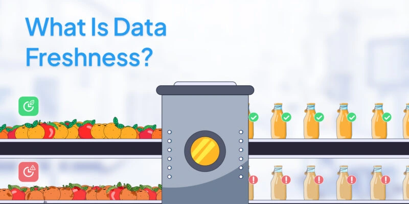
Real datasets mix numbers (price, age) with labels (city, plan, browser). Models handle numbers out of the box. Categorical features need care. A naive step — like coding cities as 0,1,2 — creates fake order and skews results. Identify nominal vs ordinal early, pick the right encoding, and plan for high cardinality and unseen values. Get this right, and categorical data becomes signal, not noise.
Types of Data in Machine Learning. What is categorical data?
Machine learning deals with various data types, but they generally fall into two broad categories: categorical and numerical. Understanding these types is a prerequisite for choosing the right preprocessing steps and algorithms. Categorical data represents groupings or labels (often text) that describe qualities or characteristics, whereas numerical data represents quantifiable amounts or counts. The figure below illustrates this classification of data types:

Numerical data comes in two forms:
- Discrete data are numeric values that are countable and often integer-valued (e.g. number of users, defect counts, inventory stock). You can list out discrete values, and there are no intermediate values between them (for instance, you can have 2 or 3 cars, but not 2.5 cars).
- Continuous data are measured on a continuous scale and can take any value within a range, often with fractional or decimal precision (e.g. height in centimeters, temperature in °C, time duration). Between any two continuous values, there are infinitely many possible values.
Categorical data can be divided into nominal and ordinal subtypes:
- Nominal data are categories without any inherent order — for example, colors (red, green, blue), product types (phone, tablet, laptop), or animal species. There is no logical ranking to these labels.
- Ordinal data, on the other hand, consist of categories with a meaningful order or rank, but the intervals between ranks are not equal. Examples include education levels (High School < Bachelor < Master < PhD), or customer satisfaction ratings (Poor < Good < Excellent). Here, Excellent is higher than Good, but we can’t say by how much.
Understanding these distinctions is crucial because different data types require different treatments. Numerical features might be scaled or normalized, whereas categorical features typically need encoding (converting categories into numeric form) before they can be used in most ML algorithms.
Nominal vs. Ordinal Data
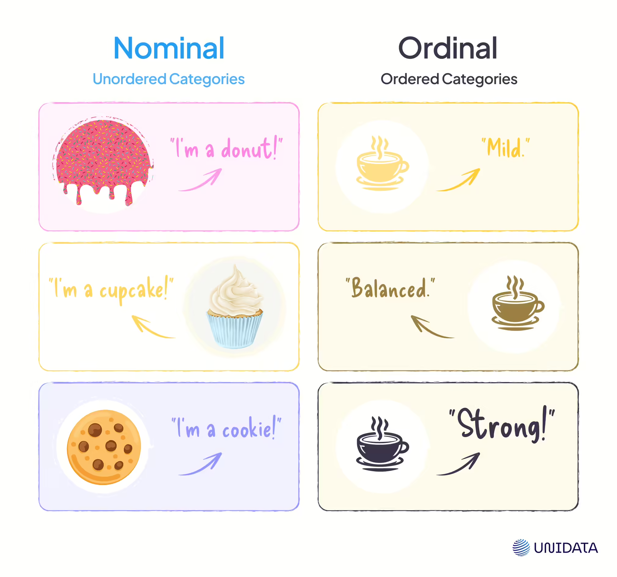
To make the distinction between nominal and ordinal data intuitive, let’s take a look at the visual above. On the left, three treats — a donut, a cupcake, and a cookie — represent nominal categories. They’re different labels with no built-in order, exactly like cities or product types in a dataset.
On the right, three coffee cups illustrate ordinal categories through increasing roast intensity: mild → balanced → strong. Here, the sequence matters. Even though we don’t assign numeric distances between these levels, the progression itself carries meaning that models can use when predicting satisfaction scores, ratings, or survey-based features.
Challenges of Categorical Data in ML
Using categorical data in machine learning presents a few key challenges.
First, as noted, most algorithms can’t directly handle non-numeric inputs. Categories like "France" or "Brazil" must be converted into numbers before feeding them to a model.
Second, naive conversion (e.g. assigning France=1, Brazil=2, Japan=3) can be problematic — the model might incorrectly interpret the numeric codes as having magnitude or order. This is especially dangerous for nominal data with no true order.
Third, categorical features can have high cardinality (many unique values). For example, a feature “Product ID” could have hundreds of distinct values. Creating a separate indicator for each can explode the feature space, making the model slow or prone to overfitting. We need smart strategies to deal with such cases (more on this later).
Finally, categories may be messy — spelling variations (“USA” vs. “U.S.A.”) or unseen categories appearing in new data can trip up a model. Handling these inconsistencies is part of the challenge.
Why do we need to encode categorical data?
Encoding is the process of converting categories into numbers so that these features can be fed into a model.
Here are the main reasons why encoding categorical data is necessary and important:
- Make inputs numeric — Most ML algorithms operate on numbers, not labels.
- Avoid false relationships — Don’t introduce fake order or distances between categories.
- Preserve true order — Keep ordinal rank (low → high) without implying equal gaps.
- Expose predictive signal — Supervised encodings can capture target-related patterns.
- Control dimensionality & sparsity — Prevent feature blow-up with many category levels.
Encoding Methods for Categorical Data
Encoding categorical values means converting them into numeric representations that machine learning models can use. There are multiple encoding techniques available, and the choice of encoding method can significantly affect model performance.
Below, we overview the most common encoding methods for categorical data.
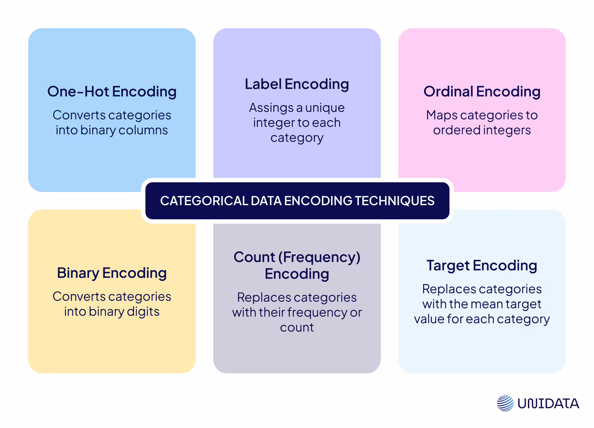
One-Hot Encoding
One-hot encoding is one of the simplest and most widely used techniques for encoding categorical data. It creates new binary features (columns) for each unique category value, and indicates presence (1) or absence (0) of that category in each observation.
Suppose a feature Weather has three possible values: Sunny, Rainy, Foggy. One-hot encoding will create three new columns (e.g., Weather_Sunny, Weather_Rainy, Weather_Foggy). For a given record, the column corresponding to its weather is set to 1 and the others to 0. For instance, a Sunny item becomes Weather_Sunny=1, Weather_Rainy=0, Weather_Foggy=0. Each row will have exactly one of these dummy columns equal to 1 (assuming each record has one category value).
When to use:
Use one-hot for categories with no natural order (city, weather, brand) and a reasonable number of values. It stops the model from thinking one label is “bigger” than another.
Advantages
- No fake order; each category becomes its own 0/1 column.
- Easy to use and well supported (pandas, scikit-learn); works with number-only models.
Limitations
- Many categories → many columns (≈ k or k–1).
- Lots of zeros (sparse), which can be heavy and hurt distance-based models.
- New categories need an “unknown” bucket or refitting the encoder.
Example — One-Hot Encoding
Let’s demonstrate one-hot encoding using pandas:
import pandas as pd
from sklearn.preprocessing import OneHotEncoder


df = pd.DataFrame({'Weather': ['Sunny', 'Rainy', 'Foggy', 'Rainy', 'Sunny']})


ohe = OneHotEncoder(sparse_output=False, handle_unknown='ignore')
X = ohe.fit_transform(df[['Weather']])


cols = ohe.get_feature_names_out(['Weather'])
encoded = pd.DataFrame(X, columns=cols, index=df.index).astype(int)
print(encoded)
Running this code would produce output like:
  Weather_Foggy  Weather_Rainy  Weather_Sunny
0             0              0              1
1              0              1              0
2              1              0              0
3              0              1              0
4              0              0              1
Label Encoding
Label encoding converts each category into a unique integer ID, but these numbers are arbitrary and do not represent any natural order. The mapping is usually alphabetical or based on how the encoder sees the data.
Example:
If Department = {Sales, HR, Finance}, a label encoder may assign:
- Finance → 0
- HR → 1
- Sales → 2
Now the original categorical column is replaced by these IDs. The key point is that 0, 1, 2 have no semantic meaning beyond being identifiers. The model should not interpret “Sales (2) > HR (1).”
When to use:
Suitable for nominal (unordered) categories, but only in models that don’t rely on numeric distances (e.g., tree-based algorithms like Decision Trees, Random Forest, XGBoost).
Advantages:
- Very compact: one integer column instead of many dummy variables.
- Easy to implement with scikit-learn.
- Works well with algorithms that split on values rather than compute distances (tree models).
Limitations:
- Adds a fake order into the data. For example, a linear regression might assume “Sales (2)” is greater than “HR (1),” which is incorrect for nominal features.
- Different datasets may assign different numbers unless you save and reuse the same fitted encoder.
- Not interpretable: the numeric IDs don’t carry meaning.
Example — Label Encoding
import pandas as pd
from sklearn.preprocessing import LabelEncoder


df = pd.DataFrame({'Department': ['Sales', 'HR', 'Finance', 'Sales', 'Finance']})
le = LabelEncoder()
df['Department_id'] = le.fit_transform(df['Department'])
print(df)
Output:
 Department  Department_id
0      Sales              2
1         HR              1
2    Finance              0
3      Sales              2
4    Finance              0
Ordinal Encoding
Ordinal encoding is similar to label encoding, but here the integers are assigned to categories in a specific, meaningful order. It’s used when categories naturally follow a ranking. The encoded numbers express relative position (Low < Medium < High), but not precise numeric distance.
Example:
If Satisfaction = {Low, Medium, High}, we can encode:
- Low → 0
- Medium → 1
- High → 2
This preserves the progression, so the model understands that High > Medium > Low. But it does not mean the gap between Low→Medium is the same as Medium→High.
When to use:
Best for ordinal features with a clear progression: satisfaction levels, education level, shirt sizes, credit ratings, service tiers.
Advantages:
- Preserves meaningful order in a compact single column.
- Simple to implement with scikit-learn (OrdinalEncoder).
- Can improve performance when order matters, as models can exploit that relationship.
Limitations:
- Numeric values may incorrectly suggest equal spacing. A linear regression will assume the difference between 0 and 1 is the same as between 1 and 2, which may not be true.
- Not safe for nominal features (like City or Product). Adding order where none exists will mislead the model.
Example — Ordinal Encoding
import pandas as pd
from sklearn.preprocessing import OrdinalEncoder


df = pd.DataFrame({'Satisfaction': ['Low', 'Medium', 'High', 'Low', 'High']})
order = [['Low', 'Medium', 'High']]
enc = OrdinalEncoder(categories=order)
df['Satisfaction_ord'] = enc.fit_transform(df[['Satisfaction']]).astype(int)
print(df)
Output:
 Satisfaction  Satisfaction_ord
0          Low                 0
1       Medium                 1
2         High                 2
3          Low                 0
4         High                 2
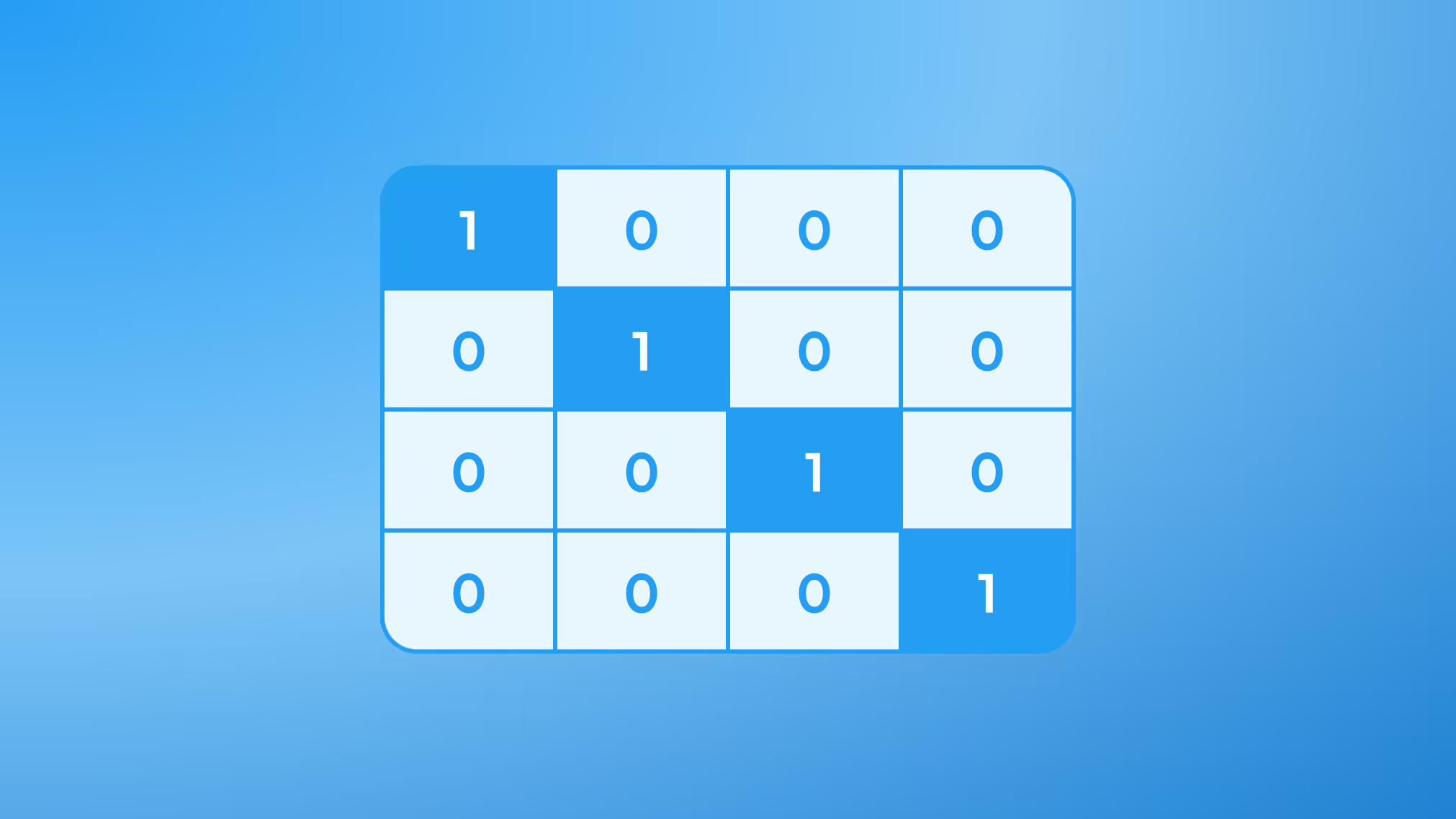
Binary Encoding
Binary encoding is a compact way to encode high-cardinality categorical features. You first map each category to an integer ID, then split that ID into binary bits across several 0/1 columns. The number of new columns grows logarithmically with the number of categories (≈ ⌈log₂ m⌉), not linearly like one-hot.
Example:
Suppose Airport_Code = {CDG, HND, JFK, LAX, SFO}.
Under the hood, the binary encoder learns a mapping from each airport code to an integer ID (based on the categories seen during fit), computes the bit width as ⌈log₂(5)⌉ = 3, converts each ID to a 3-bit binary string, and outputs three 0/1 columns:
CDG (0) → 000 → columns 0,0,0
HND (1) → 001 → columns = 0,0,1
JFK (2) → 010 → columns = 0,1,0
LAX (3) → 011 → columns = 0,1,1
SFO (4) → 100 → columns = 1,0,0
You get 3 columns instead of 5 one-hot columns; for dozens/hundreds of airports, the savings grow quickly.
When to use:
Use binary encoding when a feature has many unique values (dozens or hundreds). It cuts columns far more than one-hot, avoids fake order, and works well with many ML models.
Advantages
- Far fewer columns than one-hot.
- Less memory, often faster to train.
- Keeps some similarity between categories (shared bits).
Limitations
- More complex to set up; usually needs a library.
- Hard to read: bit columns don’t map cleanly to labels.
- May group categories by accident; extremely high cardinality can still mean many columns.
Example — Binary encoding with pandas
!pip install category_encoders


import pandas as pd
import category_encoders as ce


data = pd.DataFrame({'Airport_Code': ['JFK', 'SFO', 'LAX', 'CDG', 'HND', 'SFO', 'JFK']})


encoder = ce.BinaryEncoder(cols=['Airport_Code'])


encoded = encoder.fit_transform(data)


result = pd.concat([data, encoded], axis=1)
print(result)
Output:
Airport_Code  Airport_Code_0  Airport_Code_1  Airport_Code_2
0          JFK               0               0               1
1          SFO               0               1               0
2          LAX               0               1               1
3          CDG               1               0               0
4          HND               1               0               1
5          SFO               0               1               0
6          JFK               0               0               1
Count (Frequency) Encoding
Count encoding (or frequency encoding) replaces each category with the number of times (or frequency) it appears in the dataset. For example, if in a dataset City=Austin appears 3 times, City=Boston 2 times, City=Chicago 1 time, we encode:
- Austin → 3
- Boston → 2
- Chicago → 1
When to use:
Use count encoding when how often a category appears can help prediction, especially with many unique values. It also avoids a huge one-hot matrix.
Advantages:
- Simple and fast.
- One numeric column.
- Keeps the “common vs rare” signal.
- Saves memory for high-cardinality features.
Limitations:
- Loses the actual category; different categories with the same count look the same.
- If frequency doesn’t relate to the target, it adds noise.
- Counts depend on the dataset and can drift; not for ordinal data.
Example — Count (Frequency) Encoding:
import pandas as pd
import category_encoders as ce


df = pd.DataFrame({'City': ['Austin', 'Boston', 'Austin', 'Chicago', 'Boston', 'Austin']})


ce_enc = ce.CountEncoder(cols=['City'])
df_enc = ce_enc.fit_transform(df)


print(pd.concat([df, df_enc], axis=1))
Output:
    City  City
0   Austin     3
1   Boston     2
2   Austin     3
3   Chicago    1
4   Boston     2
5   Austin     3
Target Encoding
Target encoding (also known as mean encoding or likelihood encoding) replaces each category with a statistic of the target for that category — most commonly the mean.
Example: predicting fraud with MerchantID. If, in training data, MerchantID="M42" has fraud rate 0.27, you encode all M42 rows as 0.27 for that feature. This injects learned signal about how each category relates to the target.
When to use:
Use target encoding for supervised tasks with many categories when one-hot would be too wide and the category likely affects the label. Fit on training data only and validate to avoid leakage.
Advantages:
- Captures category-to-target signal and can boost accuracy.
- One dense numeric column per feature instead of many sparse ones.
Limitations:
- Easy to overfit, especially for rare categories; needs smoothing and out-of-fold encoding.
- More complex to set up than one-hot; mistakes cause leakage.
- Not for unsupervised tasks; mappings can drift if the data changes.
Example — Target Encoding (Mean Encoding)
import pandas as pd
from category_encoders import TargetEncoder


# Sample data
df = pd.DataFrame({
    'city': ['Moscow', 'London', 'Moscow', 'Paris', 'London', 'Paris', 'Moscow'],
    'bought': [1, 0, 1, 0, 1, 0, 1]  # target variable
})


print("Original data:")
print(df)


# Target Encoding
encoder = TargetEncoder(cols=['city'])
df_encoded = encoder.fit_transform(df['city'], df['bought'])


print("\nAfter Target Encoding:")
print(df_encoded.head())
Recap of Encoding Choices
As a summary, here’s when to consider each method:
| Method | Best for |
|---|---|
| One-hot encoding | Nominal features with a manageable number of levels (e.g., City, Brand). |
| Label encoding | Nominal features only when using tree-based models (IDs treated as labels, not magnitudes). |
| Ordinal encoding | Ordinal features with a true ranking (e.g., Low < Medium < High; Basic < Pro < Enterprise). |
| Binary encoding / Hashing | High-cardinality nominal features (dozens/hundreds of levels) where one-hot is too wide (e.g., ZipCode, SKU, MerchantID). |
| Frequency (Count) encoding | Cases where prevalence might carry signal; compact alternative to one-hot for high cardinality. |
| Target (Mean) encoding | Supervised tasks with predictive, high-cardinality categories and enough data/validation. |
By choosing the right encoding method based on your data’s nature and the algorithm’s requirements, you can often boost your model’s learning and generalization.
Dealing With High-Cardinality Categorical Features
High cardinality means a feature has many unique values. Think Customer ID with thousands. One-hot then creates a huge, sparse matrix. That slows training and can hurt results. Simple label IDs add little signal. They can also mislead some models.
Group rare categories. Combine infrequent values into “Other.” This cuts the number of levels. It also keeps your matrix smaller and easier to learn from.
Target encoding (with care). Replace each category with a target statistic, often the mean. Use smoothing and out-of-fold encoding. This reduces leakage and lowers overfitting risk. It keeps the feature dense and compact.
Hashing or binary encoding. Hashing maps categories into a fixed number of columns. Binary encoding uses a few bit columns per value. You lose some interpretability, but you keep width small.
Best Practices for Handling Categorical Data
Correctly encoding categorical data is not just about applying a method — it’s about understanding your data and the modeling context.
Here are some best practices and tips to ensure you handle categorical features effectively in machine learning:
Understand the Category Type (Nominal vs. Ordinal)
Always determine whether a categorical feature is nominal (unordered) or ordinal (ordered) before choosing an encoding. This guides your strategy.
- Nominal categories should generally be one-hot encoded to avoid introducing false order.
- Ordinal categories can be label encoded or mapped to numeric scales that reflect their rank.
- Using label encoding on a non-ordinal feature can inadvertently trick the model into seeing an order that isn’t there, which can degrade performance.
Handle New or Unseen Categories
Expect labels not seen in training. Use tools that ignore unknowns or add an “Unknown” bucket. With target encoding, set unseen labels to the global mean (or a smoothed value). Make sure the model doesn’t crash or guess wildly.
Avoid Overfitting with Target-Based Encodings
Fit encodings on training only. Use out-of-fold encoding and smoothing to reduce leakage. Never look at test data. Rare categories need extra shrinkage.
Watch Out for Sparsity and Distance Metrics
One-hot is sparse. k-NN and k-means rely on distances and can behave poorly. Prefer denser encodings (target, embeddings) or use a better distance metric.
Leverage Model-Specific Capabilities
CatBoost and LightGBM can handle categoricals natively. Trees tolerate label IDs; linear models and neural nets need numeric features. For deep learning, use embeddings for very large vocabularies.
Combine Encoding with Feature Engineering
Group similar categories to cut levels. Break features into useful parts (e.g., year, month). Add interactions only when needed — they can explode feature count.
Conclusion
Categorical data describes membership or quality, not amount. It is common in ML. Handle it well so models can use names and labels. With the right preprocessing, models read categories correctly. Accuracy and reliability improve. Categorical features can be as useful as numbers.
Frequently Asked Questions (FAQ)
Categorical data represents labels such as city, product category, or satisfaction level. Nominal features have no order, while ordinal features have a meaningful ranking. Choosing the correct encoding (one-hot, label, ordinal encoding) ensures models treat categories correctly and don’t learn false relationships.
Principal Component Analysis (PCA) is designed for continuous numerical variables and doesn’t work directly with raw categorical features. Even after encoding, PCA is rarely ideal because it assumes linear variance structures. Better alternatives for categorical variables include feature hashing, binary encoding, embeddings, or target encoding for high-cardinality features.
Yes — certain Naive Bayes variants work with categorical inputs.
- Multinomial Naive Bayes handles discrete counts and encoded categories.
- Bernoulli Naive Bayes works with binary features like one-hot encoded variables.
- Gaussian Naive Bayes is not suitable for purely categorical data.
With proper encoding, Naive Bayes can model categorical variables effectively.
- One-hot encoding — nominal features with few categories.
- Ordinal encoding — ordered categories.
- Binary or hashing encoding — high-cardinality variables.
- Target encoding — supervised tasks with strong category-to-target signal.
Selecting the right method improves performance across tree-based models, linear models, neural networks, and LLM-powered tabular systems.